3  Data Cleaning and Transformation

3.1 Introduction

In this lesson, we’ll tackle the often-messy reality of real-world data: dirty data. We’ll learn how to identify common data quality issues like missing values, outliers, and inconsistencies, and then apply techniques in R to clean and transform the data into a usable format. This lesson will also focus on cloud deployments with version control.

3.2 Learning Objectives

  • Identify common data quality issues.
  • Detect missing values and apply appropriate handling methods (removal, imputation).
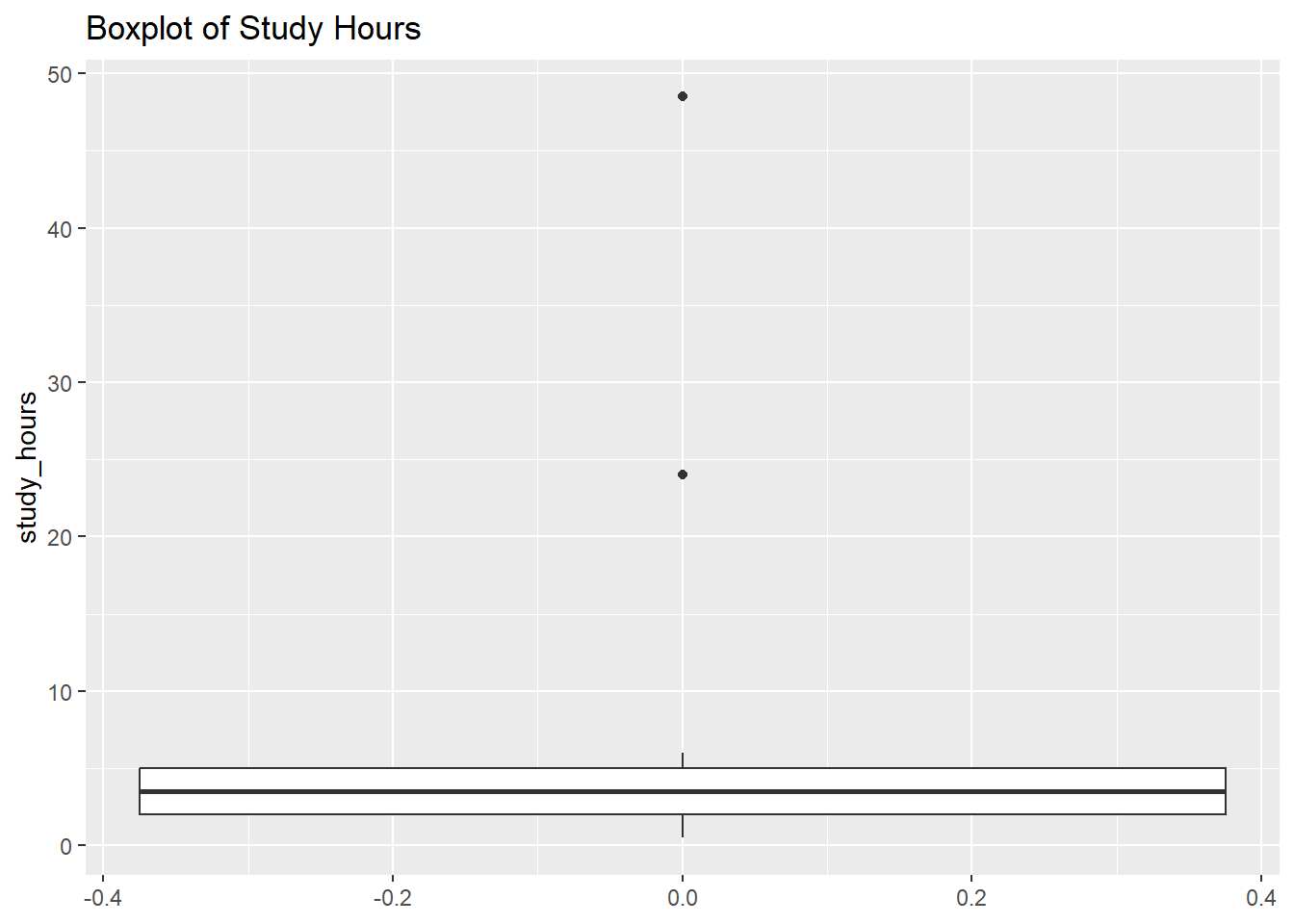
  • Detect outliers and apply appropriate handling methods (trimming, capping, transformation).
  • Correct inconsistent data entries (e.g., typos, inconsistent formatting).
  • Commit and upload the project again to version control.

3.3 What is Dirty Data?

Dirty data refers to data that is inaccurate, incomplete, inconsistent, or otherwise unreliable. Common sources of dirty data include:

  • Human error during data entry
  • Data integration issues from multiple sources
  • Software bugs
  • Inconsistent data standards

3.4 The exam_scores Dataset: Let’s Get Specific

We’ll use our exam_scores dataset (or a modified version with intentional errors) to illustrate these cleaning techniques. We’ll assume the dataset contains columns like:

  • student_id: Unique identifier for each student.
  • study_hours: Number of hours spent studying.
  • score: Exam score (out of 100).
  • grade: Letter grade (A, B, C, D, F).

3.5 Identifying Data Quality Issues

  1. Missing Values (NA):

    • Let’s check for missing values in the score column:
    library(tidyverse)
Warning: package 'tidyverse' was built under R version 4.2.3
Warning: package 'ggplot2' was built under R version 4.2.3
Warning: package 'tibble' was built under R version 4.2.3
Warning: package 'tidyr' was built under R version 4.2.3
Warning: package 'readr' was built under R version 4.2.3
Warning: package 'purrr' was built under R version 4.2.3
Warning: package 'dplyr' was built under R version 4.2.3
Warning: package 'stringr' was built under R version 4.2.3
Warning: package 'forcats' was built under R version 4.2.3
Warning: package 'lubridate' was built under R version 4.2.3
── Attaching core tidyverse packages ──────────────────────── tidyverse 2.0.0 ──
✔ dplyr     1.1.2     ✔ readr     2.1.4
✔ forcats   1.0.0     ✔ stringr   1.5.0
✔ ggplot2   3.4.3     ✔ tibble    3.2.1
✔ lubridate 1.9.2     ✔ tidyr     1.3.0
✔ purrr     1.0.2     
── Conflicts ────────────────────────────────────────── tidyverse_conflicts() ──
✖ dplyr::filter() masks stats::filter()
✖ dplyr::lag()    masks stats::lag()
ℹ Use the conflicted package (<http://conflicted.r-lib.org/>) to force all conflicts to become errors
    exam_scores <- read.csv("https://raw.githubusercontent.com/sijuswamyresearch/R-for-Data-Analytics/refs/heads/main/data/exam_scores.csv")

    sum(is.na(exam_scores))
[1] 1

cleaning the NAs

#Remove NA values in Exam Scores
exam_scores <- na.omit(exam_scores)
exam_scores
   student_id study_hours score grade
2           2         5.0    88     B
3           3         1.0    52     F
4           4         3.0    76     c
5           5         4.0    82     B
6           6         2.0   100     C
7           7         6.0    95     A
8           8         1.5    58     F
9           9         3.5    79     C
10         10         4.5    85     B
11         11         2.5    73     C
12         12         5.5    91     A
13         13         0.5    45     f
14         14         3.0    77     C
15         15         4.0    83     B
16         16        24.0    68     C
17         17         6.0    96     A
18         18         1.0    55     F
19         19         3.5    10     B
20         20         4.5    86     B
21         21         2.5    74     C
22         22         5.5    92     A
23         23         0.5    48     F
24         24         3.0    78     C
25         25         4.0    84     B
26         26         2.0    69     C
27         27         6.0    97     A
28         28         1.0    56     F
29         29         3.5    81     B
30         30        48.5    87     b
  1. Outliers:

    • Let’s identify potential outliers in the study_hours column using a boxplot:
    ggplot(exam_scores, aes(y = study_hours)) +
      geom_boxplot() +
      labs(title = "Boxplot of Study Hours")

    • We can then calculate the IQR and identify values outside the typical range:
    Q1 <- quantile(exam_scores$study_hours, 0.25)
    Q3 <- quantile(exam_scores$study_hours, 0.75)
    IQR <- Q3 - Q1
    
    lower_bound <- Q1 - 1.5 * IQR
    upper_bound <- Q3 + 1.5 * IQR
    
    outliers <- exam_scores %>%
      filter(study_hours < lower_bound | study_hours > upper_bound)
    
    print(outliers)
      student_id study_hours score grade
    1         16        24.0    68     C
    2         30        48.5    87     b
  2. Inconsistent Data:

    • Let’s check for inconsistent grade entries (e.g., lowercase “a” instead of uppercase “A”):
    unique(exam_scores$grade) #See if the dataset has what you expect
    [1] "B" "F" "c" "C" "A" "f" "b"

3.6 Handling Missing Values

  1. Removal: Let’s remove rows where the exam score is NA.

    exam_scores_no_na <- exam_scores %>%
      filter(!is.na(score))
  2. Imputation: We can use a simple ifelse statement to impute with the mean.

    • Mean/Median Imputation: Replace with the mean or median of the column.
    exam_scores <- exam_scores %>%
      mutate(score = ifelse(is.na(score), mean(score, na.rm = TRUE), score))

3.7 Handling Outliers

We can handle those extreme scores to help reduce the variability of the dataset.

  1. Capping (Winsorizing):

    # Cap values above the 95th percentile for study hours.
    upper_threshold <- quantile(exam_scores$study_hours, 0.95)
    exam_scores <- exam_scores %>%
      mutate(study_hours = ifelse(study_hours > upper_threshold, upper_threshold, study_hours))
    print(exam_scores)
       student_id study_hours score grade
    2           2         5.0    88     B
    3           3         1.0    52     F
    4           4         3.0    76     c
    5           5         4.0    82     B
    6           6         2.0   100     C
    7           7         6.0    95     A
    8           8         1.5    58     F
    9           9         3.5    79     C
    10         10         4.5    85     B
    11         11         2.5    73     C
    12         12         5.5    91     A
    13         13         0.5    45     f
    14         14         3.0    77     C
    15         15         4.0    83     B
    16         16        16.8    68     C
    17         17         6.0    96     A
    18         18         1.0    55     F
    19         19         3.5    10     B
    20         20         4.5    86     B
    21         21         2.5    74     C
    22         22         5.5    92     A
    23         23         0.5    48     F
    24         24         3.0    78     C
    25         25         4.0    84     B
    26         26         2.0    69     C
    27         27         6.0    97     A
    28         28         1.0    56     F
    29         29         3.5    81     B
    30         30        16.8    87     b

3.8 Correcting Inconsistent Data

Text Cleaning: Let’s apply some cleaning techniques to ensure the dataset is formatted as best as possible.

    library(stringr)

    exam_scores <- exam_scores %>%
      mutate(grade = str_to_upper(grade))

    print(unique(exam_scores$grade)) #Check if things are good now!
[1] "B" "F" "C" "A"