7  Statistical Methods for Evaluation

7.1 Introduction

In this section, we will cover statistical methods used for evaluating data and validating hypotheses. Knowing the different types of statistical tests to perform will be critical for your own dataset.

7.2 Learning Objectives

  • Explain the purpose of performing statistical tests.
  • Identify what kind of data types to use for statistical tests.
  • Create a new working git branch with statistical tests

7.3 What is a statistical test?

Statistical methods are used to interpret the data. It can include data cleaning, transformation and finding the right models or methods to test.

Some statistical tests are meant to understand the distributions of data. Other types of statistical tests are meant to compare one distribution against another, or to see if there is a relationships between the dataset.

7.3.1 Types of Data that work best with different tests

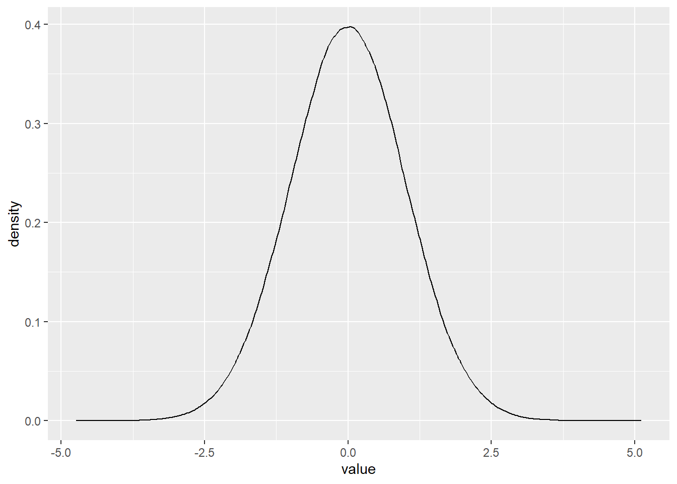
Different data formats have unique distributions, which are important to understand before performing any statistical tests. Tests like T-Tests work best with normal-style data, which has to be manually created. Also, there are tests that can convert data into a numerical result to run another test.

For this exercise we will discuss the common types of tests:

  • Normal test Normal test involves checking a statistical assumption. One of the most common checks is the normality assumption.

  • T-test Allows for 2 means to be compared. The most common type involves the use of numerical values to perform a comparison.

  • Pearson Test Determines how strong a relationship is between 2 distributions

  • Chi-squared Test: Use for evaluating the relationship between 2 categorical features.

7.3.2 Performing a Normal Statistical Test

In general, to create a normal set of distributions, you can use a built in function, for example rnorm to quickly create a normal distribution. Here’s how to create the data and to run a “Normal test” to validate the data:

  1. Create Dataset
# create a normally distributed population set
population_norm <- data.frame(value = rnorm(n = 1000000, mean = 0, sd = 1))
summary(population_norm)
     value          
 Min.   :-4.741244  
 1st Qu.:-0.675133  
 Median :-0.000582  
 Mean   :-0.000347  
 3rd Qu.: 0.674785  
 Max.   : 5.110437  
library(ggplot2)
Warning: package 'ggplot2' was built under R version 4.2.3
#Visualize distribution, from previous steps.
ggplot(population_norm, aes(value)) +
  geom_density()

  1. Testing of normality of the data
shapiro.test(population_norm$value[1:5000]) #Run the test.

    Shapiro-Wilk normality test

data:  population_norm$value[1:5000]
W = 0.99967, p-value = 0.6156

If the p-value is less than the significance level (alpha) you reject the null hypothesis and it means there is a statistical significance. In this case, reject null. The shapiro test is testing if the data “normal”. But in this case if the test passes it has to be rejected, since it will be testing if data is “non-normal”, thus the need to invert the value.

7.3.3 Performing a t- Test

A t-test can be very useful in checking if 2 samples have differences. Here’s how you would run a t-Test.

library(tidyverse)
Warning: package 'tidyverse' was built under R version 4.2.3
Warning: package 'tibble' was built under R version 4.2.3
Warning: package 'tidyr' was built under R version 4.2.3
Warning: package 'readr' was built under R version 4.2.3
Warning: package 'purrr' was built under R version 4.2.3
Warning: package 'dplyr' was built under R version 4.2.3
Warning: package 'stringr' was built under R version 4.2.3
Warning: package 'forcats' was built under R version 4.2.3
Warning: package 'lubridate' was built under R version 4.2.3
── Attaching core tidyverse packages ──────────────────────── tidyverse 2.0.0 ──
✔ dplyr     1.1.2     ✔ readr     2.1.4
✔ forcats   1.0.0     ✔ stringr   1.5.0
✔ lubridate 1.9.2     ✔ tibble    3.2.1
✔ purrr     1.0.2     ✔ tidyr     1.3.0
── Conflicts ────────────────────────────────────────── tidyverse_conflicts() ──
✖ dplyr::filter() masks stats::filter()
✖ dplyr::lag()    masks stats::lag()
ℹ Use the conflicted package (<http://conflicted.r-lib.org/>) to force all conflicts to become errors
# Create two different populations
population1 <- data.frame(value = rnorm(n = 50, mean = 0, sd = 1), group = "A")
population2 <- data.frame(value = rnorm(n = 50, mean = .5, sd = 1), group = "B")

# Combine populations
population_combined <- rbind(population1, population2)
tble=table(population_combined$group)
barplot(tble)

library(dplyr)

# mean of samples
# Calculate mean of samples over group
mean_by_group <- population_combined %>%
  group_by(group) %>%
  summarize(mean_value = mean(value))

print(mean_by_group)
# A tibble: 2 × 2
  group mean_value
  <chr>      <dbl>
1 A        -0.0159
2 B         0.583 

Perform t Test. Note, that for this particular function, you will need at least 2 variable.

t.test(data = population_combined, value ~ group)

    Welch Two Sample t-test

data:  value by group
t = -3.0912, df = 91.211, p-value = 0.002644
alternative hypothesis: true difference in means between group A and group B is not equal to 0
95 percent confidence interval:
 -0.9837332 -0.2140628
sample estimates:
mean in group A mean in group B 
    -0.01585964      0.58303835 

From here the t-test is the main value to look for, which validates whether the averages are different. The important detail here is the p-value. As mentioned earlier, if the P-Value is less than the alpha, which is typically 0.05, it means that we should reject that distribution.

7.3.4 Performing a correlation Test

Correlation test will help find any relationships within the data. The most common type of test is the Pearson Test.

#Create data with relationships
library(tidyverse)
set.seed(123)
x = rnorm(100)
data <- data.frame(
  x,
  y = 2*x + rnorm(100)
)
#data
cor(data)
          x         y
x 1.0000000 0.8786993
y 0.8786993 1.0000000

Correlation between the two variables can be tested using the pearson corelation test.

cor.test(data$x, data$y, method = "pearson")

    Pearson's product-moment correlation

data:  data$x and data$y
t = 18.222, df = 98, p-value < 2.2e-16
alternative hypothesis: true correlation is not equal to 0
95 percent confidence interval:
 0.8246011 0.9168722
sample estimates:
      cor 
0.8786993 

Looking at the information, the details for Pearson tests show a “correlation” value.

7.3.5 Performing a chi-squared Test

The Chi-squared test is used to determine if there is a statistically significant association between two categorical variables. It’s used when you have data organized in a contingency table (a cross-tabulation of two categorical variables).

Hypotheses:

  • Null Hypothesis (H0): There is no association between the two categorical variables.
  • Alternative Hypothesis (H1): There is an association between the two categorical variables.

Here’s how to perform a Chi-squared test in R:

  1. Create a Contingency Table: Create a cross-tabulation of the two categorical variables.
library(tidyverse)

# Create a sample dataset 
data <- data.frame(
  gender = factor(rep(c("Male", "Female"), times = c(40, 70))),
  smoker = factor(rep(c("Yes", "No"), times = c(60, 50)))
)

# Create a contingency table
contingency_table <- table(data$gender, data$smoker)
print(contingency_table)
        
         No Yes
  Female 50  20
  Male    0  40

Performing chi-squared test.

# Perform the Chi-squared test
chi_squared_test <- chisq.test(contingency_table)
print(chi_squared_test)

    Pearson's Chi-squared test with Yates' continuity correction

data:  contingency_table
X-squared = 49.54, df = 1, p-value = 1.944e-12

Interpreting the Results:

The output of chisq.test() will provide the following information:

  • Chi-squared Statistic: A measure of the difference between the observed and expected frequencies.
  • Degrees of Freedom: Reflects the number of independent pieces of information used in the test.
  • P-value: The probability of obtaining the observed results (or more extreme results) if the null hypothesis is true.
    • A small P-value indicates that the null hypothesis is unlikely to be true.
  • Decision: If the p-value is less than or equal to the significance level (alpha), you reject the null hypothesis.
    • If p-value <= alpha, reject the null hypothesis.
    • If p-value > alpha, fail to reject the null hypothesis.