4Lab Session 3: Symbolic operations in Laplace Transform
4.1 Experiment 5: The Laplace Transform and Frequency Response
The Laplace Transform is a powerful mathematical tool used extensively in circuit analysis, control systems, and signal processing. It transforms a function from the time domain, \(f(t)\), into the frequency domain, \(F(s)\).
While this is useful for solving differential equations, its true power in engineering comes from analyzing the frequency response. By setting the complex variable \(s = j\omega\) (where \(j\) is the imaginary unit and \(\omega\) is angular frequency), we can see how a system or signal behaves at different frequencies. This is analyzed through two key plots: the Magnitude Plot and the Phase Plot.
4.1.1 Aim
To compute the Laplace transform of given functions and, most importantly, to visualize and interpret their frequency response through magnitude and phase plots.
4.1.2 Objectives
To use Python’s SymPy library for symbolic Laplace transforms.
To understand how to obtain the frequency response function \(F(j\omega)\) from the Laplace transform \(F(s)\).
To generate and interpret magnitude and phase plots.
To connect these plots to physical concepts like amplification, attenuation, and time delay (phase shift).
4.1.3 Algorithm
Define Symbols: Use sp.symbols() to declare symbolic variables t (time), s (Laplace variable), and w (frequency, \(\omega\)).
Define the Function: Specify the time-domain function \(f(t)\) as a symbolic expression.
Compute Laplace Transform: Use sp.laplace_transform() to find the corresponding \(F(s)\).
Derive Frequency Response: Substitute \(s = j\omega\) into the symbolic expression for \(F(s)\) to get the frequency response function \(F(j\omega)\).
Prepare for Plotting: Convert the symbolic expressions for \(f(t)\) and \(F(j\omega)\) into fast numerical functions using sp.lambdify().
Generate Data:
Create a numerical array of time points t_values.
Create a logarithmic array of frequency points w_values using np.logspace().
Calculate the complex values of \(F(j\omega)\) for the frequency range.
Calculate Magnitude and Phase:
Magnitude: np.abs(F_jw_values)
Phase: np.angle(F_jw_values, deg=True) (in degrees for easier interpretation)
Plot: Create three subplots: the time-domain signal, the magnitude plot (log-log scale), and the phase plot (log-x scale). This set of frequency plots is known as a Bode Plot.
4.1.4 Case Study: An RC Low-Pass Filter’s Impulse Response
Problem: The voltage response of a simple RC low-pass filter to a sharp input (an impulse) is an exponential decay function, \(f(t) = e^{-at}\), where \(a = 1/RC\). Let’s analyze this signal for \(a=1\).
Physical Interpretation: * Magnitude |F(jω)|: Tells us how much the filter will pass or block a sine wave of frequency \(\omega\). * Phase arg(F(jω)): Tells us how much the filter will delay a sine wave of frequency \(\omega\).
Code
import sympy as spimport numpy as npimport matplotlib.pyplot as plt# --- 1. Define symbols ---t, s, w = sp.symbols('t s w', real=True, positive=True)a = sp.Symbol('a', real=True, positive=True)# --- 2. Define the function ---f = sp.exp(-a*t)# --- 3. Compute Laplace Transform ---F_s = sp.laplace_transform(f, t, s, noconds=True)# --- Set parameter for our specific case ---f_case = f.subs(a, 1)F_s_case = F_s.subs(a, 1)# --- 4. Derive Frequency Response ---F_jw = F_s_case.subs(s, 1j* w)# --- Print the symbolic results ---print(f"Function: f(t) = {f_case}")print(f"Laplace Transform: F(s) = {F_s_case}")print(f"Frequency Response: F(jω) = {F_jw}")# --- 5. Lambdify for numerical evaluation ---f_func = sp.lambdify(t, f_case, 'numpy')F_jw_func = sp.lambdify(w, F_jw, 'numpy')# --- 6. & 7. Generate Data and Calculate Mag/Phase ---t_values = np.linspace(0, 5, 400)f_values = f_func(t_values)w_values = np.logspace(-1, 2, 400) # From 0.1 to 100 rad/sF_jw_values = F_jw_func(w_values)magnitude = np.abs(F_jw_values)phase = np.angle(F_jw_values, deg=True)# --- 8. Plotting ---plt.figure(figsize=(10, 8))# Plot f(t)plt.subplot(3, 1, 1)plt.plot(t_values, f_values, color='blue')plt.title('Time Domain: $f(t) = e^{-t}$ (Impulse Response of RC Filter)')plt.xlabel('Time (t)')plt.ylabel('Amplitude')plt.grid(True)# Plot Magnitude |F(jω)|plt.subplot(3, 1, 2)plt.loglog(w_values, magnitude, color='red')plt.title('Frequency Response: Magnitude Plot')plt.xlabel('Frequency (ω) [rad/s]')plt.ylabel('|F(jω)| (Gain)')plt.grid(True, which="both", ls="-")# Plot Phase arg(F(jω))plt.subplot(3, 1, 3)plt.semilogx(w_values, phase, color='purple')plt.title('Frequency Response: Phase Plot')plt.xlabel('Frequency (ω) [rad/s]')plt.ylabel('Phase (degrees)')plt.grid(True, which="both", ls="-")plt.tight_layout()plt.show()
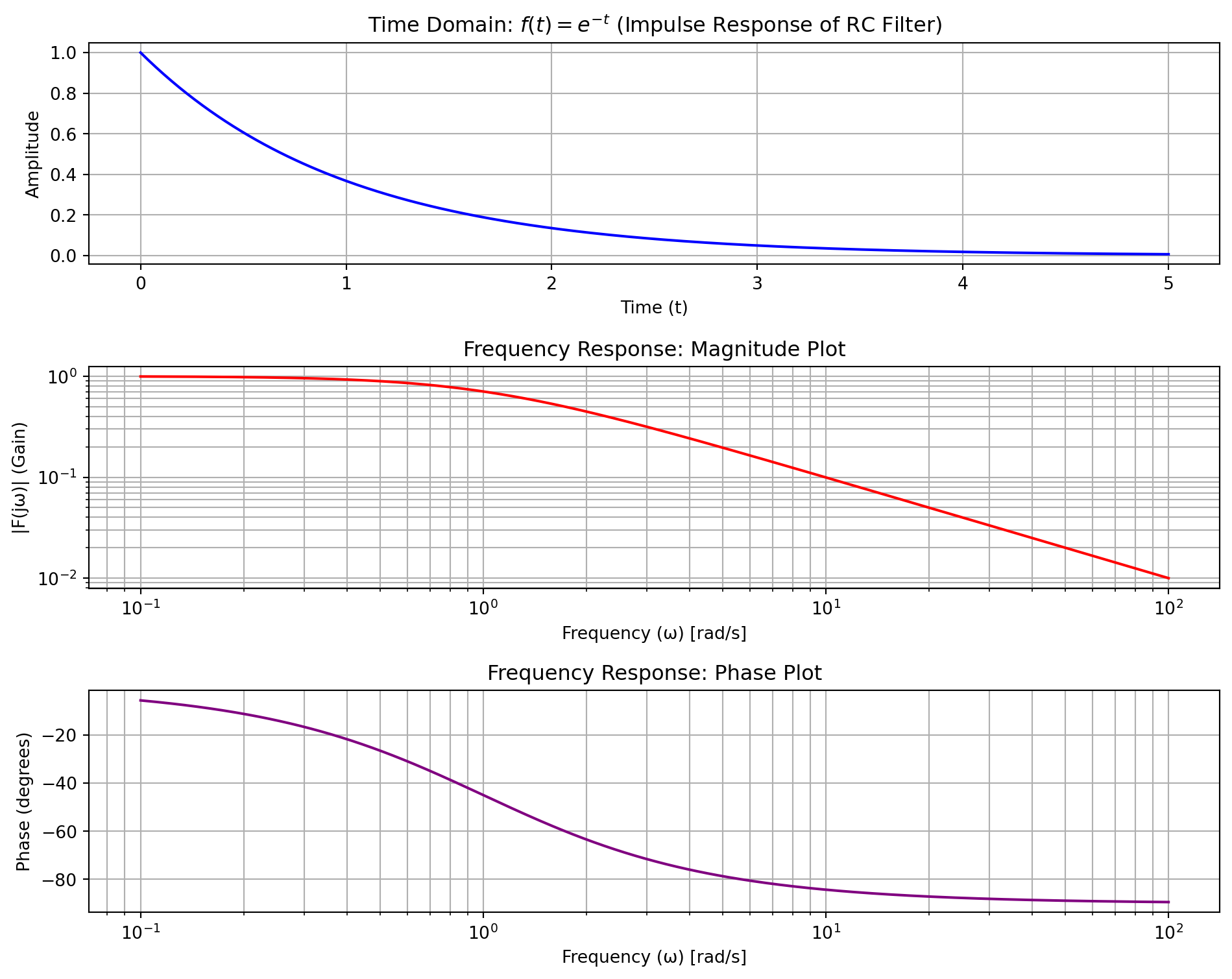
Figure 4.1: Time-domain plot of an exponential decay and its corresponding Bode Plot (Magnitude and Phase).
4.1.5 Results and Discussion
Time Domain: The function \(e^{-t}\) shows a sharp start at 1, followed by a slow decay.
Magnitude Plot: This plot clearly shows the behavior of a low-pass filter. At low frequencies (e.g., \(\omega<1\)), the magnitude (gain) is close to 1, meaning these signals are passed through without attenuation. As frequency increases, the magnitude rolls off, indicating that high-frequency signals are blocked. The “corner frequency” where the roll-off begins is at \(\omega=1/a=1\) rad/s.
Phase Plot: At very low frequencies, the phase shift is near 0 degrees. As the frequency approaches the corner frequency, the phase lag increases, reaching -45 degrees at \(\omega=1\) rad/s. At very high frequencies, the phase shift approaches -90 degrees, meaning a high-frequency sine wave passing through this filter will be delayed by a quarter of its cycle. This delay is a fundamental property of physical systems like filters.
4.1.6 Application Challenge 1: A Damped Oscillator
Your Task: Analyze a signal representing a damped sine wave, which is characteristic of many mechanical and electrical systems that oscillate but lose energy over time (e.g., a mass on a spring with friction, or an RLC circuit). The function is given by: \(f(t)=e^{-at}\sin(\omega t)\). Use the following parameters: \(a = 0.5\) (Damping factor), \(\omega_0 =5\) rad/s (Natural oscillation frequency). Follow the full algorithm to produce the time-domain plot and the full Bode plot (magnitude and phase).
Solution to the Application Challenge
Code
# --- Define symbols and parameters ---t, s, w = sp.symbols('t s w', real=True, positive=True)a = sp.Symbol('a', real=True, positive=True)w0 = sp.Symbol('w0', real=True, positive=True)# --- Define the function ---f_damped = sp.exp(-a*t) * sp.sin(w0*t)# --- Compute its Laplace Transform using the frequency shift theorem ---# The transform of e^(-at)f(t) is F(s+a)F_s_damped = sp.laplace_transform(sp.sin(w0*t), t, s)[0].subs(s, s + a)# --- Set parameters for our specific case ---params = {a: 0.5, w0: 5}f_case_damped = f_damped.subs(params)F_s_case_damped = F_s_damped.subs(params)# --- Derive Frequency Response ---F_jw_damped = F_s_case_damped.subs(s, 1j* w)# --- Print the symbolic results ---print(f"Function: f(t) = {f_case_damped}")print(f"Laplace Transform: F(s) = {sp.simplify(F_s_case_damped)}")print(f"Frequency Response: F(jω) = {F_jw_damped}")# --- Lambdify for numerical evaluation ---f_damped_func = sp.lambdify(t, f_case_damped, 'numpy')F_jw_damped_func = sp.lambdify(w, F_jw_damped, 'numpy')# --- Generate Data ---t_values = np.linspace(0, 8, 500)f_values = f_damped_func(t_values)w_values = np.logspace(-1, 2, 500)F_jw_values = F_jw_damped_func(w_values)magnitude = np.abs(F_jw_values)phase = np.angle(F_jw_values, deg=True)# --- Plotting (with raw strings for all labels) ---plt.figure(figsize=(10, 8))plt.subplot(3, 1, 1)plt.plot(t_values, f_values, color='blue')plt.title(r'Time Domain: Damped Sine Wave $f(t) = e^{-0.5t} \sin(5t)$')plt.xlabel(r'Time (t)')plt.ylabel(r'Amplitude')plt.grid(True)plt.subplot(3, 1, 2)plt.loglog(w_values, magnitude, color='red')plt.title(r'Frequency Response: Magnitude Plot')plt.axvline(x=5, color='gray', linestyle='--', label=r'Natural Freq.($\omega_{0}$=5)')plt.xlabel(r'Frequency ($\omega$)[rad/s]')plt.ylabel(r'|F(j$\omega$)|(Gain)')plt.legend()plt.grid(True, which="both", ls="-")plt.subplot(3, 1, 3)plt.semilogx(w_values, phase, color='purple')plt.title(r'Frequency Response: Phase Plot')plt.axvline(x=5, color='gray', linestyle='--', label=r'Natural Freq.($\omega_{0}$=5)')plt.xlabel(r'Frequency ($\omega$)[rad/s]')plt.ylabel(r'Phase (degrees)')plt.legend()plt.grid(True, which="both", ls="-")plt.tight_layout()plt.show()
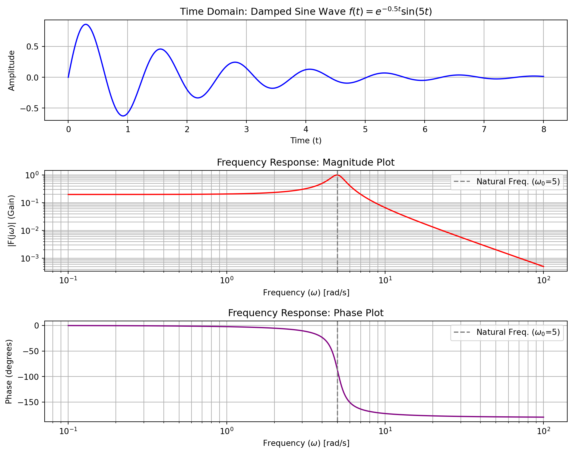
Figure 4.2: Analysis of a damped sine wave, showing a resonant peak in its frequency response.
Discussion of Challenge Solution
Time Domain: The signal is a sine wave whose amplitude decays exponentially over time, which is exactly what we expect from the function.
Magnitude Plot: This plot shows a clear resonant peak. The gain is highest for input frequencies very close to the system’s natural oscillation frequency, \(\omega_0=5\) rad/s. This means if you “excite” this system with a frequency of 5 rad/s, it will respond with the largest amplitude. This phenomenon is critical in understanding both mechanical resonance (e.g., why soldiers break step on bridges) and electrical resonance (e.g., tuning a radio).
Phase Plot: The phase experiences a very rapid shift of 180 degrees around the resonant frequency. It starts at 0 degrees (for very low frequencies), drops sharply to -180 degrees through the resonance point, indicating a complete inversion of the signal’s phase. This sharp phase change is a key indicator of resonance in a system.
Result
By focusing on magnitude and phase, this experiment provides us with a much deeper and more practical understanding of the Laplace transform’s role in engineering.
4.1.7 Application Challenge 2: Combined Decay and Ramp Signal
Your Task: Consider a signal that represents the voltage in a circuit with both a discharging capacitor component and a linearly increasing input voltage. The combined signal is given by: \[
f(t) = A e^{-\alpha t} + B t
\]
Compute and visualize the Laplace transform and frequency response for this function using the following parameters:
A = 5 (Initial amplitude of the exponential decay)
\(\alpha = 2\) (Decay rate)
B = 3 (Slope of the ramp function)
Follow the full algorithm to produce the time-domain plot and the full Bode plot (magnitude and phase).
4.1.8 Solution to the Application Challenge 2
Here is the complete Python code to solve the application challenge. We’ll analyze how the combination of a decaying signal and a constantly growing ramp signal appears in the frequency domain.
Code
# --- Define symbols and parameters ---import sympy as spimport numpy as npimport matplotlib.pyplot as pltt, s, w = sp.symbols('t s w', real=True, positive=True)A, alpha, B = sp.symbols('A alpha B', real=True, positive=True)# --- Define the function ---f_combined = A * sp.exp(-alpha * t) + B * t# --- Compute its Laplace Transform ---# SymPy can handle the sum directly due to the linearity of the transformF_s_combined = sp.laplace_transform(f_combined, t, s)[0]# --- Set parameters for our specific case ---params = {A: 5, alpha: 2, B: 3}f_case_combined = f_combined.subs(params)F_s_case_combined = F_s_combined.subs(params)# --- Derive Frequency Response ---F_jw_combined = F_s_case_combined.subs(s, 1j* w)# --- Print the symbolic results ---print(f"Function: f(t) = {f_case_combined}")# We can use simplify to combine the terms into a single fractionprint(f"Laplace Transform: F(s) = {sp.simplify(F_s_case_combined)}")print(f"Frequency Response: F(jω) = {F_jw_combined}")# --- Lambdify for numerical evaluation ---f_combined_func = sp.lambdify(t, f_case_combined, 'numpy')F_jw_combined_func = sp.lambdify(w, F_jw_combined, 'numpy')# --- Generate Data ---t_values = np.linspace(0, 3, 400)f_values = f_combined_func(t_values)# Frequency range for plotting (logarithmic scale)w_values = np.logspace(-1, 2, 400) # From 0.1 to 100 rad/sF_jw_values = F_jw_combined_func(w_values)# Calculate Magnitude and Phasemagnitude = np.abs(F_jw_values)phase = np.angle(F_jw_values, deg=True)# --- Plotting ---plt.figure(figsize=(10, 8))# Plot f(t)plt.subplot(3, 1, 1)plt.plot(t_values, f_values, color='blue')plt.title(r'Time Domain: $f(t) = 5e^{-2t} + 3t$')plt.xlabel(r'Time (t)')plt.ylabel(r'Amplitude')plt.grid(True)# Plot Magnitude |F(jω)|plt.subplot(3, 1, 2)plt.loglog(w_values, magnitude, color='red')plt.title(r'Frequency Response: Magnitude Plot')plt.xlabel(r'Frequency ($\omega$)[rad/s]')plt.ylabel(r'|F(j$\omega$)|(Gain)')plt.grid(True, which="both", ls="-")# Plot Phase arg(F(jω))plt.subplot(3, 1, 3)plt.semilogx(w_values, phase, color='purple')plt.title(r'Frequency Response: Phase Plot')plt.xlabel(r'Frequency ($\omega$)[rad/s]')plt.ylabel(r'Phase (degrees)')plt.grid(True, which="both", ls="-")plt.tight_layout()plt.show()
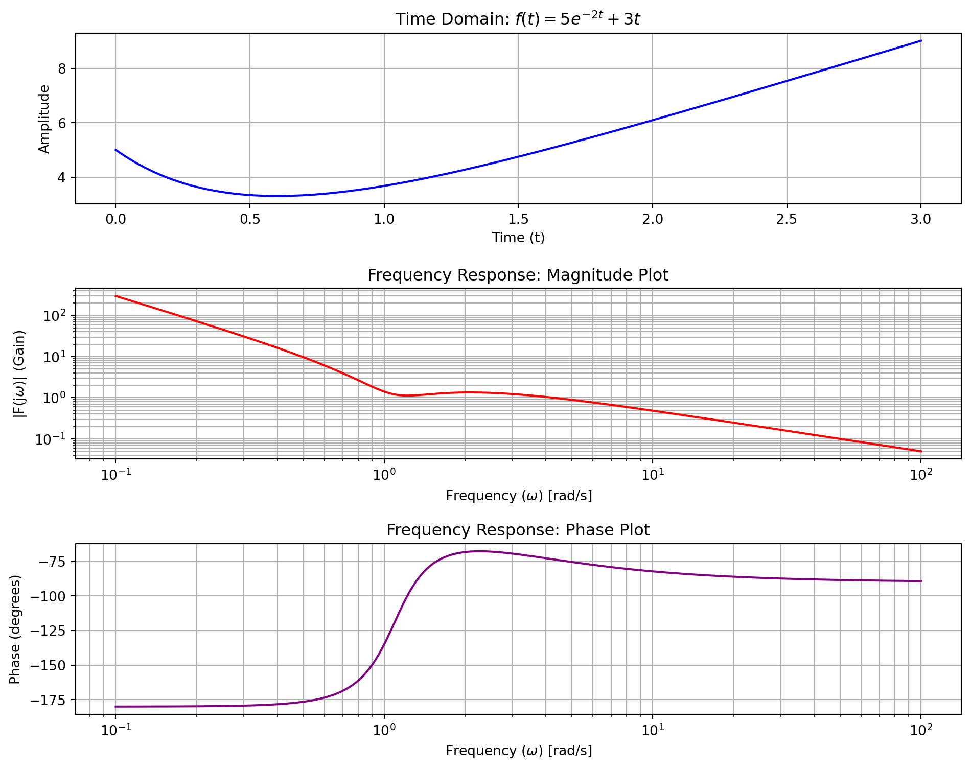
Figure 4.3: Analysis of a combined exponential decay and ramp signal.
4.1.8.1 Results and Discussion of the Challenge
The symbolic computation confirms that the Laplace transform of \(f(t)=5e^{-2t}+3t\) is, \(F(s)=\frac{5}{s^2+2}+\frac{2}{s^2}\). The frequency analysis reveals how these two components interact.
Time-Domain Plot: The plot shows the function starting at an amplitude of 5 (from the \(Ae^{-at}\) term). For a short time, the function’s value decreases as the exponential decay is stronger than the ramp’s growth. However, as t increases, the decay term vanishes and the ramp term (\(3t\)) dominates, causing the signal to increase linearly.
Magnitude Plot: The magnitude plot is dominated by the ramp function at low frequencies. The \(\frac{1}{s^2}\) term in the transform results in a very high magnitude as \(\omega \to 0\). This is because a ramp is a signal with infinite energy concentrated at the lowest frequencies (it never stops growing). The plot shows a steep roll-off, characteristic of this term. The influence of the exponential term \(\frac{5}{s+2}\) is seen as a “shoulder” in the plot around \(\omega=2\) rad/s, but it’s a minor feature compared to the ramp’s overwhelming low-frequency content.
Phase Plot: The phase plot is particularly interesting. At very low frequencies, the phase approaches -180 degrees. This is a direct consequence of the \(\frac{1}{s^2}\) term from the ramp. In the frequency domain, \(s^2\to (j\omega)^2\to -\omega^2\). A negative real number has a phase of -180 degrees (or +180). As frequency increases, the phase begins to rise, influenced by the other term in the transform, whose phase is between 0 and -90 degrees. This shows the complex interplay between the phase characteristics of the two combined signals.
This analysis demonstrates how the frequency response can deconstruct a complex time-domain signal, revealing the distinct spectral “fingerprints” of its constituent parts.
4.2 Experiment 6: The Inverse Laplace Transform
After analyzing a system or signal in the frequency domain, we often need to return to the time domain to understand the actual physical behavior—how voltage changes, how a robot arm moves, etc. The Inverse Laplace Transform, denoted \(\mathcal{L}^{-1}\{F(s)\}\), accomplishes this, converting a function \(F(s)\) back into its time-domain equivalent, \(f(t)\).
4.2.1 Aim
To compute the Inverse Laplace transform of given s-domain functions and to visualize the connection between the frequency-domain characteristics and the resulting time-domain signal.
4.2.2 Objectives
To use SymPy to calculate the inverse Laplace transform of a given function \(F(s)\).
To analyze the frequency response (magnitude and phase) of the given \(F(s)\).
To plot the resulting time-domain function \(f(t)\).
To visually connect features in the frequency domain (like resonant peaks) to behaviors in the time domain (like oscillations).
4.2.3 Algorithm
Import Libraries: Import sympy, numpy, and matplotlib.pyplot.
Define Symbols: Declare symbolic variables s, t, and w.
Define Laplace-Domain Function: Specify the s-domain function \(F(s)\) as a symbolic expression.
Analyze Frequency Response of F(s):
Substitute \(s = j\omega\) to get the frequency response function \(F(j\omega)\).
Lambdify \(F(j\omega)\) to prepare for numerical plotting.
Generate a frequency array w_values and calculate the magnitude and phase of \(F(j\omega)\).
Compute the Inverse Laplace Transform:
Use sp.inverse_laplace_transform(F, s, t)[0] to find the time-domain function \(f(t)\).
Lambdify the resulting symbolic expression \(f(t)\).
Plot and Visualize: Create a set of plots to show the full picture:
The Magnitude plot of \(F(j\omega)\).
The Phase plot of \(F(j\omega)\).
The resulting time-domain plot of \(f(t)\).
4.2.4 Case Study: An Ideal Resonator
Problem: You are given the s-domain function \(F(s) = \frac{1}{s^2 + 1}\). This is the transfer function of an ideal, undamped second-order system (like a frictionless mass-spring or a lossless LC circuit). Analyze its frequency response and find its impulse response in the time domain by computing the inverse Laplace transform.
Theoretical Result: This is the classic transform pair for \(\sin(t)\).
The given F(s) is: 1/(s**2 + 1)
The computed Inverse Laplace Transform f(t) is: sin(t)
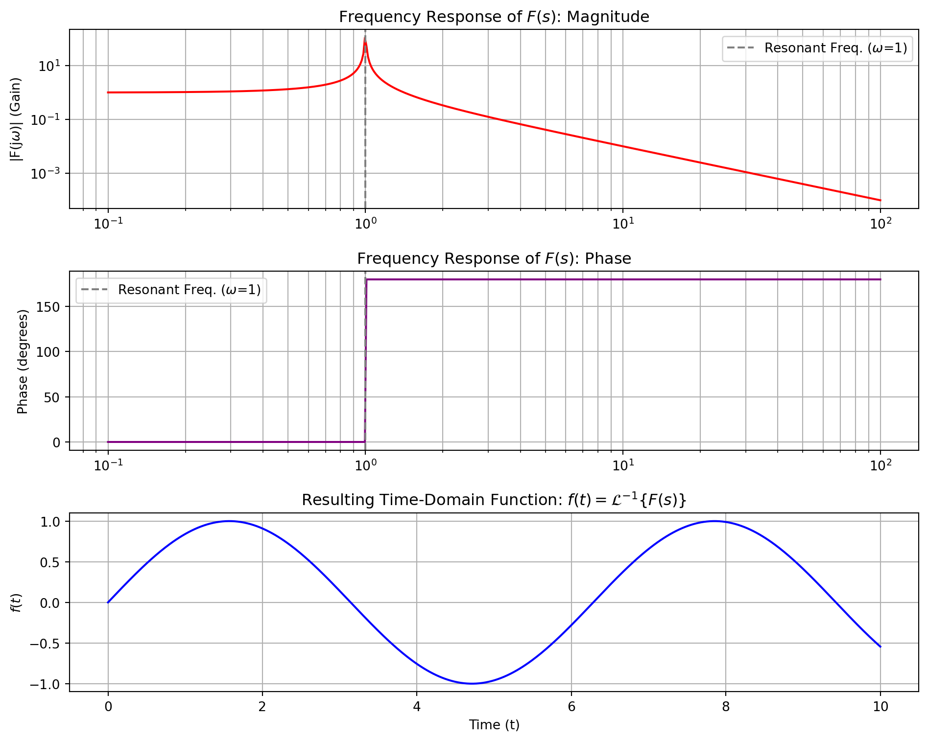
Figure 4.4: Bode Plot of F(s) = 1/(s^2+1) and its corresponding time-domain response, f(t)=sin(t).
4.2.4.1 Results and Discussion
This example provides a perfect illustration of the connection between the frequency and time domains.
Frequency Domain Analysis: The magnitude plot shows an infinitely sharp resonant peak at \(\omega=1\) rad/s. This tells us the system is extremely sensitive to inputs at this specific frequency and will have a massive response. The phase plot shows an instantaneous 180-degree flip at \(\omega=1\), another hallmark of ideal resonance.
Time Domain Result: The inverse Laplace transform correctly yields \(f(t)=sin(t)\). The plot of this function is an undamped sine wave that oscillates forever. This is the time-domain manifestation of the infinite resonant peak seen in the frequency domain. An undamped system, when “hit” by an impulse, will oscillate at its natural frequency indefinitely.
4.3 Application Challenge: Step Response of an RLC Circuit
Problem: Consider a series RLC circuit which is initially at rest (zero initial conditions). A step voltage of 5 volts is applied at \(t=0\). Determine the step response of the circuit, i.e., the current \(i(t)\) as a function of time, using the inverse Laplace transform method. Use the following component values:
Resistance (R): 10 Ω
Inductance (L): 0.1 H
Capacitance (C): 0.001 F (1 mF)
Circuit Analysis
For a series RLC circuit, Kirchhoff’s Voltage Law (KVL) gives:
\[
L \frac{di(t)}{dt} + R i(t) + \frac{1}{C} \int_0^t i(\tau) \, d\tau = v_s(t)
\]
Taking the Laplace transform of the entire equation (with zero initial conditions):
\[
sLI(s) + RI(s) + \frac{1}{sC}I(s) = V(s)
\]
The input is a step voltage of 5V, so \(v_s(t) = 5u(t)\), and its transform is \(V(s) = \frac{5}{s}\). Substituting for \(V(s)\) and solving for the current \(I(s)\):
\[
I(s) \left( sL + R + \frac{1}{sC} \right) = \frac{5}{s} \implies I(s) = \frac{\frac{5}{s}}{sL + R + \frac{1}{sC}}
\]
Simplifying this expression gives us the function we need to find the inverse transform of:
import sympy as spimport numpy as npimport matplotlib.pyplot as plt# --- Define symbols and parameters ---s, t = sp.symbols('s t', real=True, positive=True)R_val, L_val, C_val, V_val =10, 0.1, 0.001, 5# --- Define the s-domain function I(s) ---# Derived from the circuit analysis aboveI_s = (V_val / L_val) / (s**2+ (R_val / L_val) * s +1/ (L_val * C_val))print(f"The s-domain expression for the current is I(s) =")sp.pprint(I_s)# --- Compute the Inverse Laplace Transform to find i(t) ---# <<<<<<<<<<<<<<<<<<<< FIX IS HERE: Add noconds=True <<<<<<<<<<<<<<<<<<<<i_t = sp.inverse_laplace_transform(I_s, s, t, noconds=True)# ^^^^^^^^^^^^^^^^^^^^^^^^^^^^^^^^^^^^^^^^^^^^^^^^^^^^^^^^^^^^^^^^^^^^^^^^^print("\nThe time-domain expression for the current is i(t) =")sp.pprint(i_t)# --- Lambdify for plotting ---i_t_func = sp.lambdify(t, i_t, 'numpy')# --- Generate time values and plot ---t_values = np.linspace(0, 0.1, 500) # The action happens quicklyi_values = i_t_func(t_values)plt.figure(figsize=(10, 5))plt.plot(t_values, i_values, color='blue')plt.title(r'RLC Circuit Step Response: Current $i(t)$')plt.xlabel(r'Time (t)[seconds]')plt.ylabel(r'Current (i)[Amps]')plt.grid(True)plt.show()
The s-domain expression for the current is I(s) =
         50.0
──────────────────────
 2
s  + 100.0⋅s + 10000.0

The time-domain expression for the current is i(t) =
                   -50.0⋅t
0.577350269189626⋅ℯ       ⋅sin(86.6025403784439⋅t)
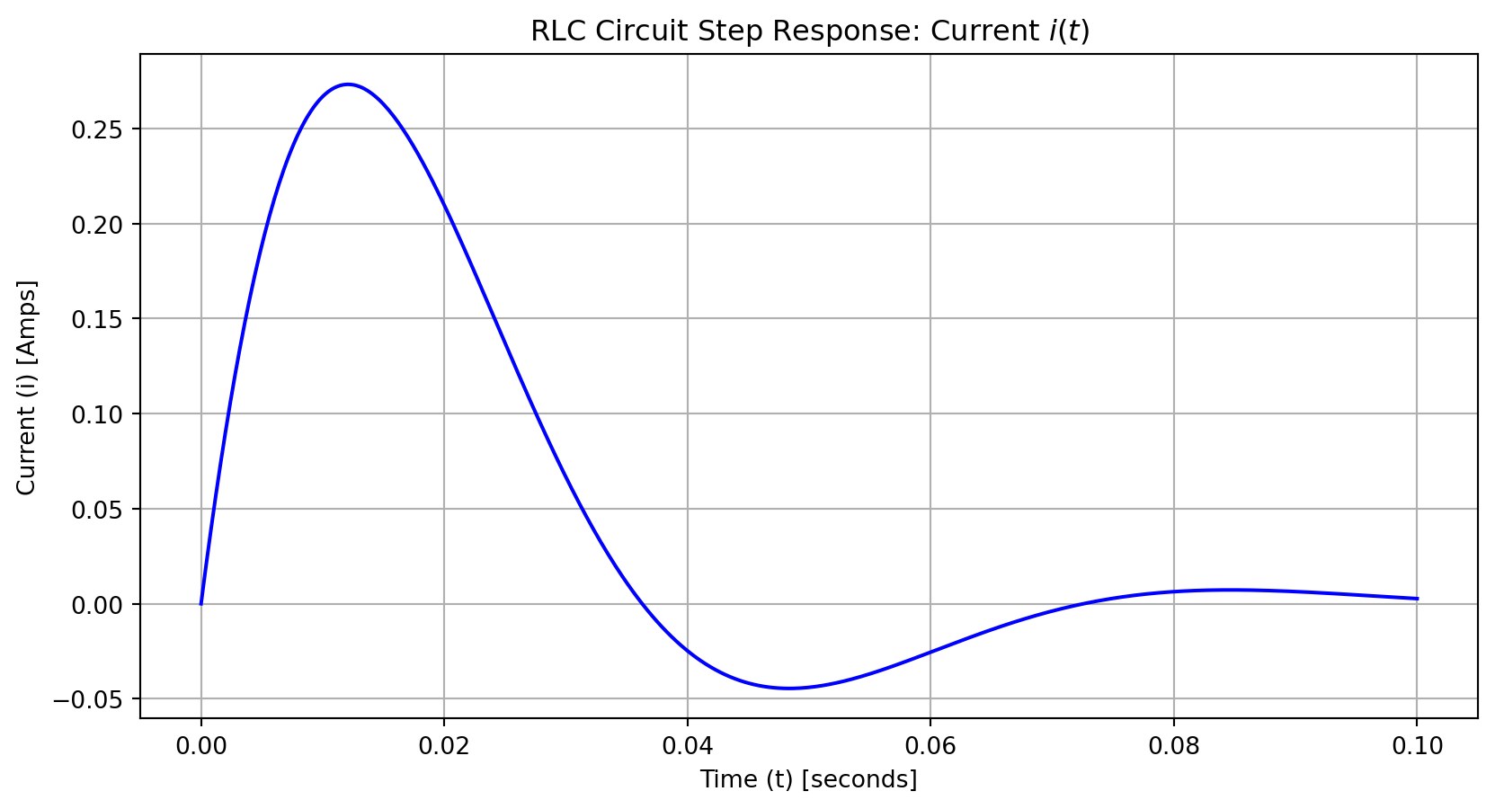
Figure 4.5: The current i(t) in an RLC circuit after a 5V step input is applied.
4.3.0.1 Discussion of RLC Circuit Result
The inverse Laplace transform provides the exact analytical solution for the current \(i(t)\) in the circuit.
Underdamped Response: The plot shows a classic underdamped response. When the voltage is applied, the current surges to a peak, overshoots the final steady-state value, and then oscillates with decreasing amplitude until it settles.
Steady-State Behavior: As \(t\to \infty\), the current \(i(t)\to 0\). This is physically correct. In a DC circuit, after the initial transient period, the inductor acts like a short circuit (a wire) and the capacitor acts as an open circuit. Since the capacitor blocks the DC current in the steady state, the final current must be zero.
Connection to System Poles: The oscillatory behavior is due to the complex conjugate poles of the denominator of \(I(s)\). If the poles were real and distinct, the response would be overdamped (no oscillation). If the poles were real and repeated, it would be critically damped. This problem beautifully demonstrates how the mathematical properties of \(F(s)\) directly dictate the physical nature of \(f(t)\).