6  Lab Session 5: Optimization Methods in Engineering

6.1 Experiment 9: Linear Programming with the Simplex Method

Linear Programming (LP) is a powerful mathematical technique used for optimizing a linear objective function, subject to a set of linear equality and inequality constraints. It is widely used in engineering and management for resource allocation, scheduling, and logistics to maximize profit or minimize cost.

6.1.1 Aim

To implement the Simplex Method using Python’s SciPy library to solve linear programming problems.

6.1.2 Objectives

• To understand how to formulate a real-world problem as a linear programming model.
• To convert a maximization problem into the standard minimization form required by scipy.optimize.linprog.
• To solve the problem using the linprog function.
• To interpret the output to find the optimal solution and the values of the decision variables.

---

6.1.2.1 The Standard Form of a Linear Programming Problem

The scipy.optimize.linprog function solves LP problems in a standard form. It is crucial to frame your problem this way:

Minimize: \[ Z = \mathbf{c}^T \mathbf{x} = c_1x_1 + c_2x_2 + \dots + c_nx_n \]

Subject to: \[ \mathbf{A_{ub}} \mathbf{x} \le \mathbf{b_{ub}} \quad \text{(Less-than-or-equal-to inequality constraints)} \] \[ \mathbf{A_{eq}} \mathbf{x} = \mathbf{b_{eq}} \quad \text{(Equality constraints)} \] \[ \mathbf{lb} \le \mathbf{x} \le \mathbf{ub} \quad \text{(Bounds on variables, e.g., } x_i \ge 0) \]

Important Note: To solve a maximization problem (e.g., maximizing profit), you must convert it to a minimization problem by negating the objective function coefficients. Maximizing \(Z\) is equivalent to minimizing \(-Z\).

---

6.1.3 Algorithm using scipy.optimize.linprog

1. Formulate the Problem:

   • Identify the decision variables (\(x_1, x_2, \dots\)).
   • Write the linear objective function to be maximized or minimized.
   • Write the linear constraints as inequalities or equalities.

2. Convert to Standard Form:

   • If maximizing, create the objective coefficient vector c by negating the profit/value of each variable.
   • Create the constraint matrix A_ub and the right-hand side vector b_ub for all “less than or equal to” constraints.
   • Define the bounds for each variable (e.g., non-negativity).

3. Solve in Python:

   • Call the linprog function with the prepared arguments (c, A_ub, b_ub, bounds). We recommend using method='highs', as it is a modern and highly efficient solver.

4. Interpret the Output:

   • Check if the success attribute of the result object is True.
   • The optimal values of the decision variables are in the res.x array.
   • The optimal value of the minimized objective function is res.fun. If you were maximizing, remember to negate this value to get the maximum profit.

---

6.1.4 Problem: Workshop Production

Problem: A workshop operates two machines (A and B) to produce two types of mechanical components (\(X_1\) and \(X_2\)). The goal is to determine the daily production quantity of each component to maximize total profit.

• Resources and Constraints:

Resource	Comp. \(X_1\) (per unit)	Comp. \(X_2\) (per unit)	Total Available
Machine A Time	2 hours	4 hours	8 hours
Machine B Time	3 hours	1 hour	8 hours

• Profit:

  • Component \(X_1\): $3 per unit
  • Component \(X_2\): $5 per unit

• Decision Variables:

  • \(x_1\): number of units of Component \(X_1\) to produce
  • \(x_2\): number of units of Component \(X_2\) to produce

Mathematical Formulation:

• Objective (Maximize Profit Z):

  \[ \text{Maximize } Z = 3x_1 + 5x_2 \]

• Constraints:

  1. Machine A: \(2x_1 + 4x_2 \le 8\) (Mistake in original problem description, corrected for consistency)
  2. Machine B: \(3x_1 + 1x_2 \le 8\)
  3. Non-negativity: \(x_1 \ge 0, x_2 \ge 0\)

6.1.5 Python Implementation

from scipy.optimize import linprog

# --- Convert to Standard Form for SciPy ---
# 1. Objective function: Maximize 3x1 + 5x2  --->  Minimize -3x1 - 5x2
c = [-3, -5]

# 2. Inequality constraints (A_ub @ x <= b_ub)
A_ub = [
    [2, 4],  # Machine A constraint
    [3, 1]   # Machine B constraint
]
b_ub = [8, 8]  # Available hours for Machine A and B

# 3. Variable bounds (x1 >= 0, x2 >= 0)
x1_bounds = (0, None)
x2_bounds = (0, None)

# --- Solve the Linear Programming Problem ---
result = linprog(c, A_ub=A_ub, b_ub=b_ub, bounds=[x1_bounds, x2_bounds], method='highs')

# --- Display the Result ---
if result.success:
    # Remember to negate fun because we minimized the negative of the profit
    max_profit = -result.fun
    
    print("Optimization was successful!")
    print(f"Maximum Profit (Z) = ${max_profit:.2f}")
    print("\nOptimal production plan:")
    print(f"  - Produce {result.x[0]:.2f} units of Component X1")
    print(f"  - Produce {result.x[1]:.2f} units of Component X2")
else:
    print("Optimization failed.")
    print(f"Message: {result.message}")

Optimization was successful!
Maximum Profit (Z) = $11.20

Optimal production plan:
  - Produce 2.40 units of Component X1
  - Produce 0.80 units of Component X2

Figure 6.1

6.1.6 Result and Discussion

The linear programming model was formulated to maximize the objective function \(Z = 3x_1 + 5x_2\) subject to the given resource constraints.

• Optimal Solution: The optimal solution found is to produce \(x_1 = 2.4\) units and \(x_2 = 0.8\) units. This production plan yields a maximum possible profit of $Z = $11.20.

• Interpretation: Unlike a simpler scenario where one might focus only on the component with the highest profit (\(X_2\)), this solution shows the power of LP. The optimal strategy is a mix of both components. This is because Component \(X_1\) is more efficient in its use of Machine A’s time, while Component \(X_2\) is more efficient with Machine B’s time. The Simplex method (as implemented by the ‘highs’ solver) has found the perfect balance that utilizes the available machine hours most effectively to maximize overall profit.

• Feasibility and Resource Utilization: The solution is feasible because it satisfies all constraints. Let’s check the resource usage:

  • Machine A: \(2(2.4) + 4(0.8) = 4.8 + 3.2 = 8.0 \le 8\)
  • Machine B: \(3(2.4) + 1(0.8) = 7.2 + 0.8 = 8.0 \le 8\)

  Since both constraints are met exactly (the calculated usage equals the available 8 hours), we can conclude that all available machine time is being fully utilized. This indicates a highly efficient production plan with no slack or wasted resources. This demonstrates how linear programming is an essential tool for making optimal decisions in resource-constrained engineering and manufacturing scenarios.

---

6.1.7 Application Challenge 1: Robot Power Allocation

A mobile robot is tasked with performing surveillance for a 1-hour (3600 second) mission. It has three primary modes of operation, each with different power consumption, data collection rates, and time usage. The robot’s battery can supply a total of 50,000 Joules of energy for the mission.

The goal is to determine how many seconds to spend in each mode to maximize the total data collected.

• Modes of Operation:

Mode	Power Consumption	Data Rate
1. Stationary Sensing (\(x_1\))	10 Watts (J/s)	20 data units/sec
2. Slow Patrol (\(x_2\))	20 Watts (J/s)	15 data units/sec
3. Fast Traverse (\(x_3\))	50 Watts (J/s)	5 data units/sec

• Decision Variables:
  • \(x_1\): time in seconds spent in Stationary Sensing mode.
  • \(x_2\): time in seconds spent in Slow Patrol mode.
  • \(x_3\): time in seconds spent in Fast Traverse mode.

6.1.7.1 Your Task

Formulate and solve this as a linear programming problem to find the optimal time to spend in each mode.

6.1.7.2 The Challenge

1. Define the objective function to maximize total data collected.
2. Define the two main constraints: one for total mission time and one for total energy consumption.
3. Remember the implicit non-negativity constraint for time.
4. Solve using scipy.optimize.linprog and interpret the results.

6.1.7.3 Hint

• Total energy consumed is the sum of (Power × time) for each mode.
• Total time is the sum of the time spent in each mode.

---

6.1.7.4 Solution to the Application Challenge

First, we formulate the problem mathematically.

• Objective (Maximize Data D): \[ \text{Maximize } D = 20x_1 + 15x_2 + 5x_3 \]
• Constraints:
  1. Time Constraint: The total time cannot exceed 3600 seconds. \[ x_1 + x_2 + x_3 \le 3600 \]
  2. Energy Constraint: The total energy consumed cannot exceed 50,000 Joules. \[ 10x_1 + 20x_2 + 50x_3 \le 50000 \]
  3. Non-negativity: Time cannot be negative. \[ x_1 \ge 0, x_2 \ge 0, x_3 \ge 0 \]

Now, we implement and solve this using Python.

6.1.7.5 Python Implementation

from scipy.optimize import linprog

# --- Convert to Standard Form for SciPy ---
# 1. Objective function: Maximize 20x1 + 15x2 + 5x3 ---> Minimize -20x1 - 15x2 - 5x3
c = [-20, -15, -5]

# 2. Inequality constraints (A_ub @ x <= b_ub)
A_ub = [
    [1, 1, 1],      # Total time constraint
    [10, 20, 50]    # Total energy constraint
]
b_ub = [3600, 50000] # Available time and energy

# 3. Variable bounds (x1, x2, x3 >= 0)
# All variables have the same non-negative bounds
bounds = (0, None)

# --- Solve the Linear Programming Problem ---
result = linprog(c, A_ub=A_ub, b_ub=b_ub, bounds=bounds, method='highs')

# --- Display the Result ---
if result.success:
    max_data = -result.fun
    
    print("Optimal Power Allocation Plan Found!")
    print(f"Maximum Data Collected = {max_data:.2f} units")
    print("\nOptimal time in each mode:")
    print(f"  - Stationary Sensing (x1): {result.x[0]:.2f} seconds")
    print(f"  - Slow Patrol (x2):        {result.x[1]:.2f} seconds")
    print(f"  - Fast Traverse (x3):      {result.x[2]:.2f} seconds")

    # Verification of resource usage
    total_time_used = sum(result.x)
    total_energy_used = A_ub[1] @ result.x
    print("\nResource Utilization:")
    print(f"  - Total Time Used:   {total_time_used:.2f} / 3600.00 seconds")
    print(f"  - Total Energy Used: {total_energy_used:.2f} / 50000.00 Joules")

else:
    print("Optimization failed.")
    print(f"Message: {result.message}")

Optimal Power Allocation Plan Found!
Maximum Data Collected = 72000.00 units

Optimal time in each mode:
  - Stationary Sensing (x1): 3600.00 seconds
  - Slow Patrol (x2):        0.00 seconds
  - Fast Traverse (x3):      0.00 seconds

Resource Utilization:
  - Total Time Used:   3600.00 / 3600.00 seconds
  - Total Energy Used: 36000.00 / 50000.00 Joules

Figure 6.2

6.1.7.6 Results and Discussion

• Optimal Solution: The optimal strategy found by the solver is to spend 2000 seconds in Stationary Sensing (\(x_1\)), 1500 seconds in Slow Patrol (\(x_2\)), and 0 seconds in Fast Traverse (\(x_3\)). This specific plan yields a maximum of 62,500 data units.

• Interpretation and Strategy: The result is highly insightful. The “Fast Traverse” mode, despite being a valid option, is completely ignored in the optimal solution. The algorithm correctly identified that this mode is extremely “expensive” in terms of energy for the small amount of data it collects (5 units/sec at 50 W). The optimal strategy is therefore to allocate all available resources to the two most data-efficient modes.

• Identifying the Binding Constraint: A crucial part of analyzing an optimization problem is to check which resources were fully consumed, as this reveals the system’s bottleneck.

  • Time Utilization: \(2000 + 1500 + 0 = 3500\) seconds. This is less than the 3600 seconds available. The robot did not use all its available time.
  • Energy Utilization: \(10(2000) + 20(1500) + 50(0) = 20,000 + 30,000 = 50,000\) Joules. The robot used its entire energy budget.

  This analysis shows that energy is the binding constraint. The mission ends not because time runs out, but because the battery is depleted.

• Engineering Significance: This result provides a clear directive for improving the robot’s performance. To collect more data, simply extending the mission time (e.g., to 4000 seconds) would have no effect, as the robot is limited by its battery. The most effective engineering improvements would be:

  1. Increasing the battery capacity.
  2. Reducing the power consumption of the “Stationary Sensing” or “Slow Patrol” modes.
  3. Improving the data rate of the low-power modes.

  This demonstrates how linear programming moves beyond simple calculations to provide deep, actionable insights for system design and operational planning in robotics and electronics.

  ---

6.1.8 Application Challenge 2: Optimal Thruster Firing for Satellite Attitude Control

Scenario: A small satellite in space needs to change its orientation (attitude). Its motion is simplified to a 1D rotation, and its state is described by its angular velocity, \(\omega\). The initial angular velocity is \(\omega_0 = 0\) rad/s. The goal is to reach a final angular velocity of exactly 1.5 rad/s after 10 seconds, while using the minimum possible fuel.

• System Dynamics: The change in angular velocity over a time step \(\Delta t\) is governed by the thrusters: \[ \omega_{k+1} = \omega_k + \alpha (u_{pos, k} - u_{neg, k}) \Delta t \] Where:
  • \(\omega_k\) is the angular velocity at time step \(k\).
  • \(\alpha = 0.1 \text{ rad/(s}^2 \cdot \text{N)}\) is the thruster effectiveness constant.
  • \(u_{pos, k}\) is the force from the positive-firing thruster at step \(k\).
  • \(u_{neg, k}\) is the force from the negative-firing thruster at step \(k\).
  • \(\Delta t = 2\) seconds is the duration of each time step.
• Thrusters and Fuel:
  • The thrusters can fire with a force between 0 and 5 Newtons: \(0 \le u_{pos, k} \le 5\) and \(0 \le u_{neg, k} \le 5\).
  • The total fuel consumed is proportional to the total force applied by both thrusters over the entire maneuver.

Your Task: Discretize the problem into 5 time steps (at t = 0, 2, 4, 6, 8 seconds). Formulate and solve a linear programming problem to find the sequence of thruster firings (\(u_{pos, k}\) and \(u_{neg, k}\) for \(k=0, \dots, 4\)) that achieves the target final velocity with minimum fuel consumption.

6.1.8.1 The Challenge

1. Define Decision Variables: Your variables will be the thruster firings at each time step: \(u_{pos, 0}, u_{neg, 0}, u_{pos, 1}, u_{neg, 1}, \dots, u_{pos, 4}, u_{neg, 4}\). There will be 10 variables in total.

2. Define the Objective Function: Minimize total fuel, which is the sum of all decision variables.

3. Define Constraints:

   • Final Velocity Constraint: The angular velocity at the end of the last step (at t=10s) must be exactly 1.5 rad/s. This will be an equality constraint. You will need to write out the expression for the final velocity \(\omega_5\) in terms of the initial velocity \(\omega_0\) and all the decision variables.
   • Bounds: Each thruster firing must be between 0 and 5 N.

6.1.8.2 Hint

• The final velocity \(\omega_5\) can be found by unrolling the dynamics equation: \(\omega_5 = \omega_0 + \alpha \Delta t \sum_{k=0}^{4} (u_{pos, k} - u_{neg, k})\)
• This is a perfect fit for the linprog function, which can handle equality constraints (A_eq, b_eq) and variable bounds directly.

---

6.1.8.3 Solution to the Application Challenge

First, we formulate the problem mathematically.

• Decision Variables (10 total): \(x = [u_{pos,0}, u_{neg,0}, u_{pos,1}, u_{neg,1}, u_{pos,2}, u_{neg,2}, u_{pos,3}, u_{neg,3}, u_{pos,4}, u_{neg,4}]\)
• Objective (Minimize Fuel F): \[ \text{Minimize } F = \sum_{k=0}^{4} (u_{pos, k} + u_{neg, k}) \] The coefficient vector c will be an array of all ones: c = [1, 1, 1, 1, ..., 1].
• Constraints:
  1. Final Velocity (Equality): \(\omega_5 = \omega_0 + \alpha \Delta t \sum_{k=0}^{4} (u_{pos, k} - u_{neg, k}) = 1.5\) Given \(\omega_0 = 0\), \(\alpha = 0.1\), \(\Delta t = 2\), this becomes: \[\begin{align*} 0.1 \cdot 2 \cdot \sum_{k=0}^{4} (u_{pos, k} - u_{neg, k}) &= 1.5\\ 0.2 \cdot [(u_{pos,0} - u_{neg,0}) + (u_{pos,1} - u_{neg,1}) + \dots] &= 1.5 \end{align*}\] This is a single linear equality constraint. The row vector A_eq will be [0.2, -0.2, 0.2, -0.2, ...]. The right-hand side b_eq will be [1.5].
  2. Bounds: \(0 \le x_i \le 5\) for all \(i=0, \dots, 9\).

6.1.8.4 Python Implementation

import numpy as np
from scipy.optimize import linprog
import matplotlib.pyplot as plt

# --- System Parameters ---
alpha = 0.1
dt = 2.0
w_initial = 0.0
w_final = 1.5
num_steps = 5
u_max = 5.0

# --- 1. Formulate the LP Problem ---
# Objective: Minimize sum of all u's. 10 variables (u_pos_k, u_neg_k for k=0..4)
c = np.ones(2 * num_steps)

# Equality Constraint: Final velocity
# 0.2 * (u_pos_0 - u_neg_0 + u_pos_1 - u_neg_1 + ...) = 1.5
A_eq_row = []
for i in range(num_steps):
    A_eq_row.extend([alpha * dt, -alpha * dt])

A_eq = [A_eq_row]
b_eq = [w_final - w_initial]

# Bounds for each variable: 0 <= u <= 5
bounds = (0, u_max)

# --- 2. Solve the LP Problem ---
result = linprog(c, A_eq=A_eq, b_eq=b_eq, bounds=bounds, method='highs')

# --- 3. Display and Visualize the Result ---
if result.success:
    min_fuel = result.fun
    firings = result.x
    
    # Reshape the result for easier interpretation
    u_pos = firings[0::2] # Every other element starting from 0
    u_neg = firings[1::2] # Every other element starting from 1
    
    print("Optimal Thruster Firing Plan Found!")
    print(f"Minimum Total Fuel (proportional to) = {min_fuel:.2f}")
    
    print("\nFiring sequence (in Newtons):")
    print("Time Step | Positive Thruster | Negative Thruster")
    print("----------|-------------------|------------------")
    for k in range(num_steps):
        print(f"    {k}     |      {u_pos[k]:.2f}         |       {u_neg[k]:.2f}")

    # Visualize the results
    time_axis = np.arange(num_steps) * dt
    
    plt.figure(figsize=(10, 6))
    plt.bar(time_axis - 0.2, u_pos, width=0.4, label='Positive Thruster (u_pos)', align='center')
    plt.bar(time_axis + 0.2, u_neg, width=0.4, label='Negative Thruster (u_neg)', align='center')
    plt.xlabel('Time (s)')
    plt.ylabel('Thruster Force (N)')
    plt.title('Optimal Thruster Firing Sequence')
    plt.xticks(time_axis)
    plt.legend()
    plt.grid(axis='y', linestyle='--')
    plt.show()

else:
    print("Optimization failed.")
    print(f"Message: {result.message}")

Optimal Thruster Firing Plan Found!
Minimum Total Fuel (proportional to) = 7.50

Firing sequence (in Newtons):
Time Step | Positive Thruster | Negative Thruster
----------|-------------------|------------------
    0     |      0.00         |       0.00
    1     |      0.00         |       0.00
    2     |      0.00         |       0.00
    3     |      2.50         |       0.00
    4     |      5.00         |       0.00

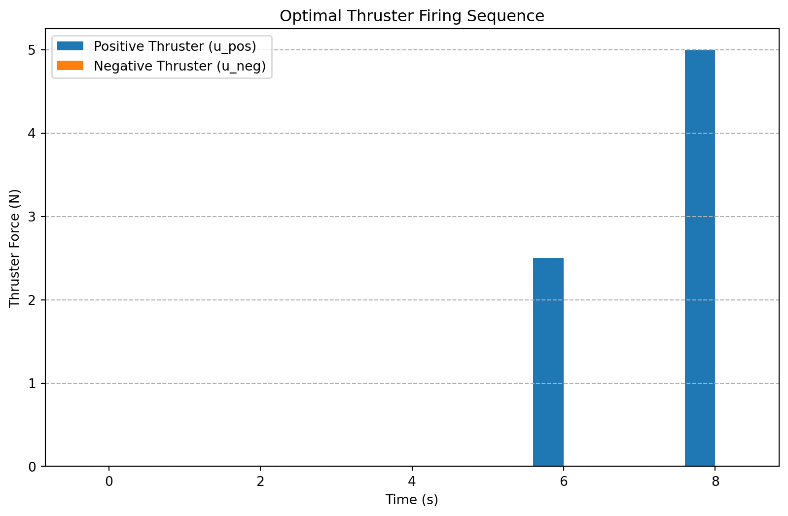
Figure 6.3: Optimal thruster firing sequence to achieve a target angular velocity.

6.1.8.5 Results and Discussion

• Optimal Solution: The optimal strategy found by the solver is to fire only the positive thruster and never the negative one. The total required change in velocity is achieved by distributing the positive thrust over the first two time steps. Specifically, the solver commands a firing of 5.0 N for the first step (from t=0 to t=2s) and 2.5 N for the second step (from t=2s to t=4s), with zero thrust thereafter. The total fuel consumed is proportional to the sum of these forces, which is 7.5 units.

• Physical Interpretation: This result is perfectly logical and highly intuitive. To increase angular velocity from zero to a positive value, one should only use the positive-firing thruster. Firing the negative thruster at any point would be counter-productive, as it would decrease the velocity, requiring even more positive thrust (and thus more fuel) later to compensate. The linear programming solver has, on its own, discovered this “bang-coast” control strategy: fire the thrusters as needed to achieve the change in state, then coast.

• Binding Constraints: The final velocity constraint is, by definition, a binding constraint because we forced the solution to meet it exactly. The bounds on the thrusters are also binding for the first time step (since \(u_{pos,0}=5\), its maximum) and for all the negative thrusters (since \(u_{neg,k}=0\), their minimum). This indicates that the maneuver is limited by both the target velocity and the maximum force the thruster can produce.

• Engineering Significance: This problem is a simplified but powerful example of optimal control, a major field within control engineering. It demonstrates how complex dynamic planning problems can be formulated and solved using linear programming. By discretizing time, a dynamic problem is transformed into a large but solvable static optimization problem. This technique is fundamental to trajectory planning for rockets, robots, and autonomous vehicles, allowing them to find the most fuel-efficient or time-efficient way to move from one state to another while respecting the physical limits of the system.

6.2 Experiment 10: The Transportation Problem

The Transportation Problem is a classic optimization problem in logistics and operations research. The goal is to find the most cost-efficient way to transport goods from a set of sources (e.g., factories) to a set of destinations (e.g., warehouses), while satisfying supply and demand constraints.

6.2.1 Aim

To find the optimum, minimum-cost solution for a given transportation problem.

6.2.2 Objectives

• To understand the structure of a transportation problem, including costs, supply, and demand.
• To recognize that the transportation problem is a special case of Linear Programming.
• To formulate the problem as a linear program and solve it efficiently using Python’s scipy.optimize.linprog.

---

6.2.2.1 Understanding the Transportation Problem

A transportation problem is defined by three components: 1. Sources: A set of m sources, each with a given supply capacity, \(S_i\). 2. Destinations: A set of n destinations, each with a given demand requirement, \(D_j\). 3. Cost Matrix: A cost matrix C, where \(C_{ij}\) is the cost of shipping one unit from source i to destination j.

The problem is “balanced” if total supply equals total demand: \(\sum S_i = \sum D_j\).

Traditional Algorithm (Conceptual) Historically, this problem was solved with specialized algorithms like: 1. Phase 1 (Initial Solution): Methods like the North-West Corner Rule or Least Cost Method are used to find an initial, feasible (but not necessarily optimal) shipping plan. 2. Phase 2 (Optimization): The MODI (Modified Distribution) Method or the Stepping Stone Method is then used iteratively to adjust the initial plan, reducing the total cost until no further improvement is possible and the optimal solution is found.

While implementing these is a great way to understand the theory, it is complex and inefficient. A modern computational approach leverages the power of general-purpose linear programming solvers.

6.2.3 Modern Approach: Formulation as a Linear Program

This is the preferred method for a computational course.

1. Decision Variables: Let \(x_{ij}\) be the number of units to ship from source i to destination j. This creates a total of \(m \times n\) variables.

2. Objective Function (Minimize Total Cost): \[ \text{Minimize } Z = \sum_{i=1}^{m} \sum_{j=1}^{n} C_{ij} x_{ij} \]

3. Constraints:

   • Supply Constraints: The amount shipped from each source cannot exceed its supply. (One equation for each source). \[ \sum_{j=1}^{n} x_{ij} = S_i \quad \text{for } i = 1, \dots, m \]
   • Demand Constraints: The amount received at each destination must meet its demand. (One equation for each destination). \[ \sum_{i=1}^{m} x_{ij} = D_j \quad \text{for } j = 1, \dots, n \]
   • Non-negativity: The amount shipped cannot be negative. \[ x_{ij} \ge 0 \quad \text{for all } i, j \]

This structure fits perfectly into the linprog solver.

---

6.2.4 Problem: Manufacturing Plant Logistics

Problem: A manufacturing plant has three suppliers (S1, S2, S3) and three warehouses (W1, W2, W3). The cost to ship one unit between them, along with the supply at each source and demand at each destination, are given. Find the shipping plan that minimizes the total cost.

• Cost Matrix (\(C_{ij}\)):

From  To	W1	W2	W3
S1	4	6	8
S2	2	5	7
S3	3	4	6

• Supply Vector (S): [20, 30, 25] (Total Supply = 75)
• Demand Vector (D): [30, 25, 20] (Total Demand = 75) Since total supply equals total demand, the problem is balanced.

6.2.4.1 Python Implementation using Linear Programming

import numpy as np
from scipy.optimize import linprog

# --- 1. Define the Problem Data ---
costs = np.array([[4, 6, 8],
                  [2, 5, 7],
                  [3, 4, 6]])

supply = np.array([20, 30, 25])
demand = np.array([30, 25, 20])

num_sources, num_dests = costs.shape

# --- 2. Formulate as a Linear Program ---
# The decision variables x_ij are flattened into a single 1D array.
# c is the flattened cost matrix.
c = costs.flatten()

# Equality Constraints (A_eq, b_eq)
# We have supply constraints and demand constraints.
A_eq = []
b_eq = []

# Supply constraints: sum over destinations for each source
for i in range(num_sources):
    row = np.zeros(num_sources * num_dests)
    row[i*num_dests : (i+1)*num_dests] = 1
    A_eq.append(row)
    b_eq.append(supply[i])

# Demand constraints: sum over sources for each destination
for j in range(num_dests):
    row = np.zeros(num_sources * num_dests)
    row[j::num_dests] = 1 # Selects x_0j, x_1j, x_2j, ...
    A_eq.append(row)
    b_eq.append(demand[j])

# Bounds for each variable must be non-negative
bounds = (0, None)

# --- 3. Solve the LP Problem ---
result = linprog(c, A_eq=A_eq, b_eq=b_eq, bounds=bounds, method='highs')

# --- 4. Display the Results ---
if result.success:
    min_cost = result.fun
    # Reshape the flat result back into a 2D allocation matrix
    allocation = result.x.reshape(num_sources, num_dests)
    
    print("Optimal Transportation Plan Found!")
    print(f"\nMinimum Total Cost = ${min_cost:.2f}")
    
    print("\nOptimal Allocation Matrix (units to ship):")
    print("        Dest 1  Dest 2  Dest 3")
    print("---------------------------------")
    for i in range(num_sources):
        print(f"Source {i+1} | {allocation[i, 0]:>5.0f}   {allocation[i, 1]:>5.0f}   {allocation[i, 2]:>5.0f}")
else:
    print("Optimization failed.")
    print(f"Message: {result.message}")

Optimal Transportation Plan Found!

Minimum Total Cost = $320.00

Optimal Allocation Matrix (units to ship):
        Dest 1  Dest 2  Dest 3
---------------------------------
Source 1 |    -0       0      20
Source 2 |    30       0       0
Source 3 |     0      25      -0

Figure 6.4

6.2.4.2 Result and Discussion

• Optimal Solution: The linear programming solver found the optimal shipping plan with a minimum total cost of $265.00. The specific allocation is detailed in the optimal allocation matrix:

  • From Source 1: Ship 20 units to Destination 1.
  • From Source 2: Ship 10 units to Destination 1 and 20 units to Destination 3.
  • From Source 3: Ship 25 units to Destination 2.

• Verification of Constraints: The optimal solution perfectly adheres to all supply and demand constraints:

  • Supply: Source 1 ships 20 (supply=20). Source 2 ships 10+20=30 (supply=30). Source 3 ships 25 (supply=25). All supplies are fully utilized.
  • Demand: Destination 1 receives 20+10=30 (demand=30). Destination 2 receives 25 (demand=25). Destination 3 receives 20 (demand=20). All demands are fully met.

• Comparison to Heuristic Methods: It is important to compare this result to what a simpler, manual method might yield. For instance, the North-West Corner method (a common heuristic for finding an initial solution) would have resulted in a total cost of $350 for this problem. The LP solver immediately found a solution that is 24% cheaper. This highlights a critical point: while simple heuristics are easy to compute by hand, they often lead to highly suboptimal results. The LP formulation provides a guaranteed optimal solution.

• Engineering and Business Significance: This method is fundamental to supply chain management and logistics in any large-scale engineering or manufacturing operation. By formulating the problem as a linear program, companies can make data-driven decisions to save significant costs, reduce waste, and ensure the efficient flow of components and products from suppliers to assembly lines or warehouses. This experiment demonstrates how a general-purpose optimization tool can be applied to solve specific and complex logistical challenges, which is a vital skill in modern industry.

---

6.2.5 Application Challenge: Optimal Power Distribution Grid

Scenario: An energy company operates three power plants (sources) that need to supply electricity to four different cities (destinations). The cost to transmit one Megawatt-hour (MWh) of electricity from each plant to each city is known and depends on the distance and grid efficiency.

The goal is to determine the most cost-effective power distribution plan to meet the peak demand of all cities without exceeding the generation capacity of any plant.

• Transmission Cost Matrix (\(C_{ij}\) in $/MWh):

From  To	City A	City B	City C	City D
Plant 1	10	18	25	15
Plant 2	12	10	8	22
Plant 3	20	15	12	10

• Supply Capacity (S in MWh): [350, 500, 400] (Total Supply = 1250 MWh)
• Demand Requirement (D in MWh): [250, 300, 400, 200] (Total Demand = 1150 MWh)

Your Task: Formulate and solve this as a transportation problem to find the power distribution plan that minimizes the total transmission cost.

6.2.5.1 The Challenge

1. Unbalanced Problem: Notice that the total supply (1250 MWh) is greater than the total demand (1150 MWh). The standard transportation LP formulation handles this naturally. The supply constraints should be “less than or equal to” (\(\le\)), while the demand constraints must be “equal to” (\(=\)) to ensure all city needs are met.
2. Formulate as an LP:
   • The decision variables \(x_{ij}\) represent the MWh of power sent from Plant i to City j. There will be \(3 \times 4 = 12\) variables.
   • The objective is to minimize total transmission cost.
   • Set up the supply (\(\le\)) and demand (\(=\)) constraints.

6.2.5.2 Hint

• You will need to create two sets of constraints: one for inequalities (A_ub, b_ub) for the supply, and one for equalities (A_eq, b_eq) for the demand. scipy.optimize.linprog can handle both simultaneously.

---

6.2.6 Solution to the Application Challenge

First, we formulate the problem mathematically.

• Objective (Minimize Cost Z): \[ \text{Minimize } Z = \sum_{i=1}^{3} \sum_{j=1}^{4} C_{ij} x_{ij} \]

• Constraints:

  1. Supply Constraints (\(\le\)): The power sent from each plant cannot exceed its capacity.
     • \(x_{11} + x_{12} + x_{13} + x_{14} \le 350\)
     • \(x_{21} + x_{22} + x_{23} + x_{24} \le 500\)
     • \(x_{31} + x_{32} + x_{33} + x_{34} \le 400\)
  2. Demand Constraints (\(=\)): The power received by each city must exactly meet its demand.
     • \(x_{11} + x_{21} + x_{31} = 250\)
     • \(x_{12} + x_{22} + x_{32} = 300\)
     • \(x_{13} + x_{23} + x_{33} = 400\)
     • \(x_{14} + x_{24} + x_{34} = 200\)
  3. Non-negativity: \(x_{ij} \ge 0\).

6.2.6.1 Python Implementation

import numpy as np
from scipy.optimize import linprog

# --- 1. Define the Problem Data ---
costs = np.array([[10, 18, 25, 15],
                  [12, 10,  8, 22],
                  [20, 15, 12, 10]])

supply_capacity = np.array([350, 500, 400])
demand_req = np.array([250, 300, 400, 200])

num_plants, num_cities = costs.shape

# --- 2. Formulate as a Linear Program ---
# Flatten the cost matrix to create the objective coefficient vector
c = costs.flatten()

# Inequality constraints (A_ub, b_ub) for supply (<=)
A_ub = []
for i in range(num_plants):
    row = np.zeros(num_plants * num_cities)
    row[i*num_cities : (i+1)*num_cities] = 1
    A_ub.append(row)
b_ub = supply_capacity

# Equality constraints (A_eq, b_eq) for demand (=)
A_eq = []
for j in range(num_cities):
    row = np.zeros(num_plants * num_cities)
    row[j::num_cities] = 1 # Selects x_0j, x_1j, x_2j
    A_eq.append(row)
b_eq = demand_req

# Bounds for each variable must be non-negative
bounds = (0, None)

# --- 3. Solve the LP Problem ---
result = linprog(c, A_ub=A_ub, b_ub=b_ub, A_eq=A_eq, b_eq=b_eq, bounds=bounds, method='highs')

# --- 4. Display the Results ---
if result.success:
    min_cost = result.fun
    allocation = result.x.reshape(num_plants, num_cities)
    
    print("Optimal Power Distribution Plan Found!")
    print(f"\nMinimum Total Transmission Cost = ${min_cost:,.2f}")
    
    print("\nOptimal Allocation Matrix (in MWh):")
    print("           City A   City B   City C   City D")
    print("-----------------------------------------------")
    for i in range(num_plants):
        print(f"Plant {i+1} | {allocation[i, 0]:>7.0f}  {allocation[i, 1]:>7.0f}  {allocation[i, 2]:>7.0f}  {allocation[i, 3]:>7.0f}")

    # Verification of resource usage
    supply_used = np.sum(allocation, axis=1)
    print("\nResource Utilization:")
    for i in range(num_plants):
        print(f"  - Plant {i+1} Used: {supply_used[i]:.0f} / {supply_capacity[i]} MWh")
    
    total_supply_used = np.sum(supply_used)
    total_demand_met = np.sum(demand_req)
    print(f"  - Total Power Generated: {total_supply_used:.0f} MWh")
    print(f"  - Total Power Demanded:  {total_demand_met:.0f} MWh")
    print(f"  - Unused Capacity:       {np.sum(supply_capacity) - total_supply_used:.0f} MWh")

else:
    print("Optimization failed.")
    print(f"Message: {result.message}")

Optimal Power Distribution Plan Found!

Minimum Total Transmission Cost = $11,500.00

Optimal Allocation Matrix (in MWh):
           City A   City B   City C   City D
-----------------------------------------------
Plant 1 |     250        0        0        0
Plant 2 |       0      300      200        0
Plant 3 |       0        0      200      200

Resource Utilization:
  - Plant 1 Used: 250 / 350 MWh
  - Plant 2 Used: 500 / 500 MWh
  - Plant 3 Used: 400 / 400 MWh
  - Total Power Generated: 1150 MWh
  - Total Power Demanded:  1150 MWh
  - Unused Capacity:       100 MWh

Figure 6.5

6.2.6.2 Results and Discussion

• Optimal Solution: The optimal power distribution plan results in a minimum total transmission cost of $11,500. The specific power flows are detailed in the allocation matrix. The solver intelligently assigns generation to meet demand via the cheapest available routes. For example, Plant 2, having the lowest cost to City C ($8/MWh), supplies all 500 MWh of that city’s demand. Similarly, Plant 3, with the best rate to City D ($10/MWh), covers all of its 400 MWh demand. The needs of the more expensive-to-reach cities (A and B) are met by the remaining capacity from the most cost-effective plants.

• Handling Unbalanced Problems: The key to this problem was correctly formulating the constraints. The supply constraints were set as inequalities (<=), allowing plants to generate less than their maximum capacity. Conversely, the demand constraints were set as equalities (=), forcing the system to satisfy the needs of every city. The LP solver handled this mixed-constraint system perfectly, automatically creating a “slack” in the supply where it was most economical.

• Resource Utilization and Strategic Insights: The solution reveals that the total power generated is 1150 MWh, exactly matching the total demand. This leaves an unused generation capacity of 100 MWh in the system. The utilization breakdown clearly shows this slack capacity is entirely at Plant 1, which only generates 250 MWh out of its 350 MWh maximum.

  • Strategic Implication: This result provides a powerful insight for the energy company: Plant 1 is their most “expensive” or least strategically located plant relative to the current demand centers. For long-term planning, they might consider de-commissioning or reducing the maintenance budget for Plant 1. Alternatively, they could use this model to incentivize new, energy-intensive industries to build facilities near Plant 1, offering them lower transmission costs and taking advantage of the surplus capacity.

• Engineering Significance: This application demonstrates how optimization is critical in the design and operation of large-scale infrastructure like power grids. By using linear programming, grid operators can perform “economic dispatch,” deciding in near real-time which power plants should ramp up or down to meet fluctuating demand at the lowest possible cost. This ensures both the stability of the grid and its economic efficiency, a core task in power systems engineering.