# Core optimization stack installation
# pip install numpy scipy matplotlib pulp pandas jupyter2 Module 1: Basics of Optimization and Linear Programming
2.1 Module Overview
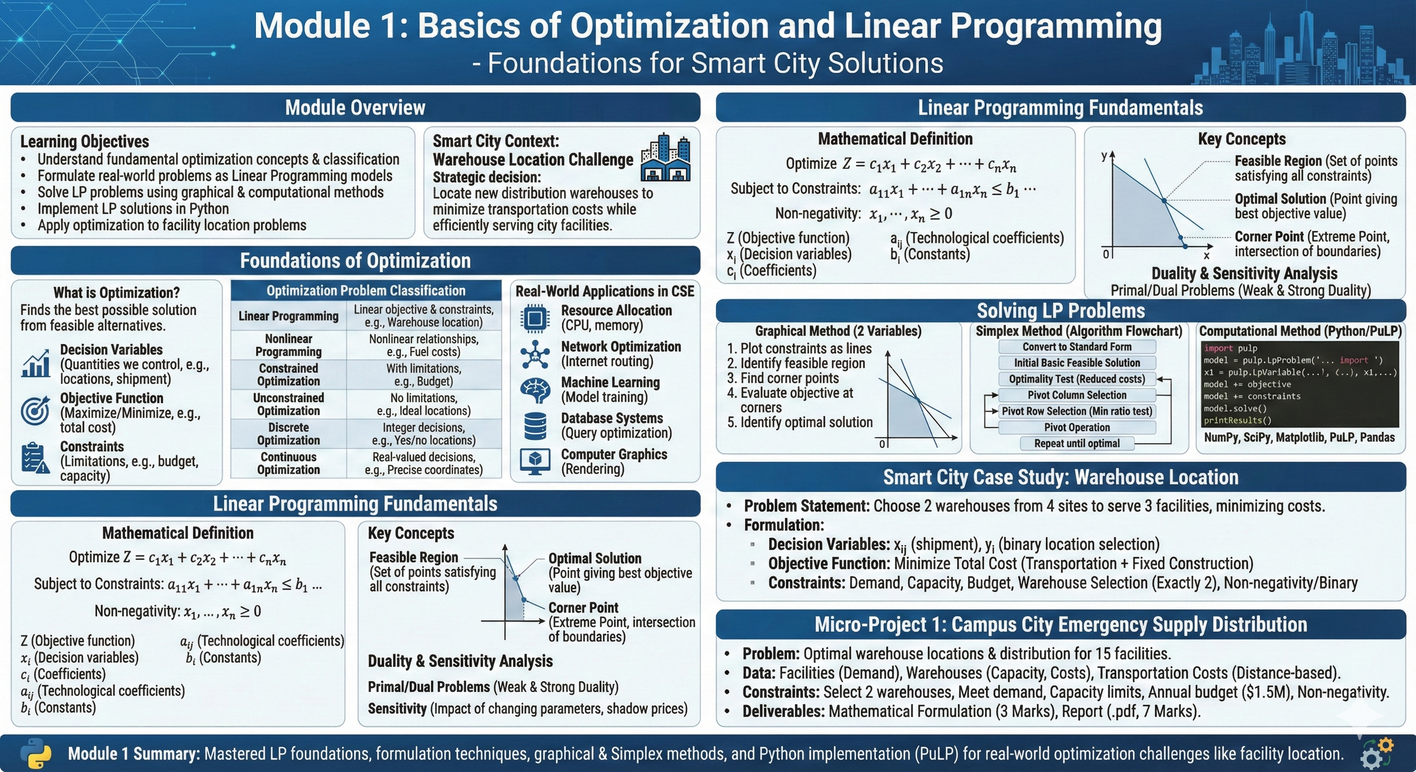
2.1.1 Learning Objectives
- Understand fundamental optimization concepts and problem classification
- Formulate real-world problems as Linear Programming models
- Solve LP problems using graphical and computational methods
- Implement LP solutions in Python for practical applications
- Apply optimization thinking to facility location problems
2.1.2 Smart City Context: Warehouse Location Challenge
In our Smart City Logistics project, we face a critical business decision: where to locate new distribution warehouses to minimize transportation costs while serving all city facilities efficiently. This module provides the mathematical foundation to solve this strategic problem.
2.2 Foundations of Optimization
2.2.1 What is Optimization?
Optimization is the science of finding the best possible solution from all feasible alternatives under given constraints. In computational terms, it involves:
- Decision Variables: Quantities we can control (e.g., warehouse locations, shipment quantities)
- Objective Function: What we want to maximize or minimize (e.g., total transportation cost)
- Constraints: Limitations and requirements (e.g., budget, capacity, demand)
2.2.2 Optimization Problem Classification
| Problem Type | Characteristics | Smart City Example |
|---|---|---|
| Linear Programming | Linear objective and constraints | Warehouse location with fixed costs |
| Nonlinear Programming | Nonlinear relationships | Fuel costs that increase with distance |
| Constrained Optimization | With limitations | Budget constraints on construction |
| Unconstrained Optimization | No limitations | Theoretical ideal locations |
| Discrete Optimization | Integer decisions | Yes/no decisions for locations |
| Continuous Optimization | Real-valued decisions | Precise coordinates for facilities |
2.2.3 Real-World Applications in CSE
- Resource Allocation: CPU time, memory allocation in operating systems
- Network Optimization: Internet routing, data flow optimization
- Machine Learning: Model training via loss function minimization
- Database Systems: Query optimization and indexing
- Computer Graphics: Rendering optimization and path tracing
2.3 Basic Python for Optimization
2.3.1 Essential Python Libraries Setup
Key
Python Libraries Required for Computational Part
NumPy: Numerical computing and array operationsSciPy: Scientific computing and optimization algorithmsMatplotlib: Data visualization and result plottingPuLP: Linear programming interfacePandas: Data manipulation and analysis
2.3.2 Python Fundamentals for Optimization
# Essential operations we'll use frequently
import numpy as np
import matplotlib.pyplot as plt

# Array operations for constraint matrices
coefficients = np.array([[2, 1], [1, 3], [4, 2]])

# Function definitions for objectives
def transportation_cost(warehouses, facilities):
    return np.sum(warehouses * facilities)

# Data handling for problem parameters
demand_data = {'Hospital': 50, 'School': 30, 'Mall': 80}
2.4 Linear Programming Fundamentals
2.4.1 Mathematical Definition of Linear Programming
A Linear Programming (LP) problem can be formally defined as:
Objective Function: \[ \text{Optimize } Z = c_1x_1 + c_2x_2 + \cdots + c_nx_n \]
Subject to Constraints:
\[ \begin{aligned} a_{11}x_1 + a_{12}x_2 + \cdots + a_{1n}x_n & \leq b_1 \\ a_{21}x_1 + a_{22}x_2 + \cdots + a_{2n}x_n & \leq b_2 \\ \vdots & \\ a_{m1}x_1 + a_{m2}x_2 + \cdots + a_{mn}x_n & \leq b_m \\ \end{aligned} \]
Non-negativity Conditions:
\[ x_1, x_2, \ldots, x_n \geq 0 \]
Where:
- \(Z\) is the objective function to be optimized (maximized or minimized)
- \(x_1, x_2, \ldots, x_n\) are the decision variables
- \(c_1, c_2, \ldots, c_n\) are the coefficients of the objective function
- \(a_{ij}\) are the technological coefficients
- \(b_1, b_2, \ldots, b_m\) are the right-hand side constants
2.4.2 Standard Forms of Linear Programming
2.4.2.1 Canonical Form (Maximization)
\[ \begin{aligned} \text{Maximize } & Z = \mathbf{c}^T\mathbf{x} \\ \text{Subject to } & \mathbf{A}\mathbf{x} \leq \mathbf{b} \\ & \mathbf{x} \geq \mathbf{0} \end{aligned} \]
2.4.2.2 Standard Form (Maximization)
\[ \begin{aligned} \text{Maximize } & Z = \mathbf{c}^T\mathbf{x} \\ \text{Subject to } & \mathbf{A}\mathbf{x} = \mathbf{b} \\ & \mathbf{x} \geq \mathbf{0} \end{aligned} \]
2.4.3 Key Concepts in Linear Programming
2.4.3.1 Feasible Region
The set of all points that satisfy all constraints simultaneously: \[ F = \{\mathbf{x} \in \mathbb{R}^n : \mathbf{A}\mathbf{x} \leq \mathbf{b}, \mathbf{x} \geq \mathbf{0}\} \]
2.4.3.2 Optimal Solution
A point \(\mathbf{x}^*\) in the feasible region that gives the best value of the objective function.
2.4.3.3 Corner Point (Extreme Point)
A point in the feasible region that cannot be expressed as a convex combination of two other distinct points in the region.
2.4.4 Smart City Case: Warehouse Location Formulation
2.4.4.1 Problem Statement
We need to choose locations for 2 warehouses from 4 potential sites to serve 3 major facilities while minimizing total costs.
2.4.4.2 Decision Variables
Let: - \(x_{ij}\): Amount shipped from warehouse \(i\) to facility \(j\) - \(y_i\): Binary variable (1 if warehouse \(i\) is built, 0 otherwise)
Where: - \(i = 1, 2, 3, 4\) (warehouse sites) - \(j = 1, 2, 3\) (facilities: Hospital, Mall, School)
2.4.4.3 Objective Function
Minimize total cost: \[ \text{Minimize } Z = \sum_{i=1}^{4} \sum_{j=1}^{3} c_{ij}x_{ij} + \sum_{i=1}^{4} f_i y_i \] Where: - \(c_{ij}\): Transportation cost per unit from warehouse \(i\) to facility \(j\) - \(f_i\): Fixed construction cost for warehouse \(i\)
2.4.4.4 Constraints
Demand Constraints (Each facility’s demand must be met): \[ \sum_{i=1}^{4} x_{ij} = d_j \quad \text{for } j = 1,2,3 \] Where \(d_j\) is the demand of facility \(j\).
Capacity Constraints (Warehouse capacity cannot be exceeded): \[ \sum_{j=1}^{3} x_{ij} \leq C_i y_i \quad \text{for } i = 1,2,3,4 \] Where \(C_i\) is the capacity of warehouse \(i\).
Budget Constraint: \[ \sum_{i=1}^{4} f_i y_i \leq B \] Where \(B\) is the total budget available.
Warehouse Selection Constraint (Select exactly 2 warehouses): \[ \sum_{i=1}^{4} y_i = 2 \]
Non-negativity and Binary Requirements: \[ x_{ij} \geq 0 \quad \text{for all } i,j \] \[ y_i \in \{0, 1\} \quad \text{for all } i \]
2.4.5 Graphical Method for Two-Variable Problems
2.4.5.1 Step-by-Step Procedure
- Plot Constraints: Convert each inequality to equality and plot the line
- Identify Feasible Region: Determine which side of each line satisfies the inequality
- Find Corner Points: Identify intersection points of constraint boundaries
- Evaluate Objective Function: Calculate objective value at each corner point
- Identify Optimal Solution: Select the corner point with best objective value
2.4.5.2 Example: Simple Warehouse Problem
Consider a simplified version with 2 warehouses and 1 facility:
Problem: \[ \begin{aligned} \text{Maximize } & Z = 40x_1 + 30x_2 \\ \text{Subject to } & 2x_1 + x_2 \leq 100 \\ & x_1 + 3x_2 \leq 90 \\ & x_1 \geq 0, x_2 \geq 0 \end{aligned} \]
Step 1: Plot Constraints - Constraint 1: \(2x_1 + x_2 = 100\) → Line through (0,100) and (50,0) - Constraint 2: \(x_1 + 3x_2 = 90\) → Line through (0,30) and (90,0)
Step 2: Identify Corner Points - Intersection of axes: (0,0), (0,30), (50,0) - Intersection of constraints: Solve: \[ \begin{aligned} 2x_1 + x_2 &= 100 \\ x_1 + 3x_2 &= 90 \end{aligned} \] Solution: \(x_1 = 42, x_2 = 16\)
Step 3: Evaluate Objective Function
- At (0,0): \(Z = 0\)
- At (0,30): \(Z = 900\)
- At (50,0): \(Z = 2000\)
- At (42,16): \(Z = 40×42 + 30×16 = 2160\)
Optimal Solution: \(x_1 = 42, x_2 = 16\) with \(Z = 2160\)
2.4.6 Simplex Method Theory
2.4.6.1 Fundamental Theorem of Linear Programming
If an LP problem has an optimal solution, then there exists at least one corner point of the feasible region that is optimal.
2.4.6.2 Simplex Algorithm Steps
Convert to Standard Form
- Convert inequalities to equations using slack variables
- Ensure all variables are non-negative
- Convert minimization to maximization if needed
Initial Basic Feasible Solution
- Identify basic variables (variables with coefficient 1 in one equation and 0 in others)
- Set non-basic variables to zero
Optimality Test
- Calculate reduced costs for non-basic variables
- If all reduced costs \(\leq 0\) (for maximization), current solution is optimal
Pivot Column Selection
- Choose non-basic variable with most positive reduced cost (for maximization)
Pivot Row Selection
- Use minimum ratio test: \(\min \left\{ \frac{b_i}{a_{ij}} : a_{ij} > 0 \right\}\)
Pivot Operation
- Make pivot element equal to 1
- Make other elements in pivot column equal to 0
Repeat until optimality condition is satisfied
2.4.6.3 Simplex Tableau Format
The simplex method uses a tableau to organize calculations:
| Basic Var | \(x_1\) | \(x_2\) | \(s_1\) | \(s_2\) | RHS |
|---|---|---|---|---|---|
| \(s_1\) | 2 | 1 | 1 | 0 | 100 |
| \(s_2\) | 1 | 3 | 0 | 1 | 90 |
| \(Z\) | -40 | -30 | 0 | 0 | 0 |
Where \(s_1, s_2\) are slack variables.
2.5 Types of Linear Programming Solutions
When we feed a problem into a solver (like the Simplex algorithm), we usually expect a single, perfect answer. But algorithms are strict logicians. If we ask for the impossible or the infinite, they will tell us exactly that. In Linear Programming, there are four distinct outcomes.
2.5.1 Unique Optimal Solution
The “Ideal” Scenario
This is the standard result. Geometrically, the feasible region is a polygon, and the Objective Function (the “slope” of profit or cost) cuts through the region such that it touches exactly one corner point (vertex) last.
- Mathematical Context: The slope of the objective function does not match the slope of any binding constraint.
- Engineering Implication: There is exactly one best way to allocate your resources. Any deviation from this plan results in lower profit or higher cost.
2.5.2 Multiple Optimal Solutions (Alternative Optima)
The “Flexibility” Scenario
Sometimes, you might get a result where the solver says: “You can choose Point A (\(x=2, y=5\)) or Point B (\(x=4, y=3\)), and the profit is exactly the same.”
- Why this happens: The slope of your Objective Function is parallel to one of the binding constraint lines. Instead of touching a single corner, the objective function lies flat against an entire edge of the feasible region.
- Engineering Implication: This is actually great news for a designer! It means you have flexibility. Mathematically, the cost is the same, but maybe Plan A is politically easier to implement than Plan B. You can choose based on secondary factors (like aesthetics or risk) without losing optimality.
2.5.3 Unbounded Solution
The “Too Good to Be True” Scenario
Imagine writing a program to maximize profit, and the output is Infinity. While exciting, this is invariably a modeling error.
- Why this happens: The feasible region is not closed (it extends infinitely in one direction), and you are trying to maximize in that direction. You have forgotten a constraint.
- Real-world Example: “Maximize production.” If you don’t add a constraint for “Available Raw Materials” or “Factory Capacity,” the math assumes you can produce infinite units.
- Mathematical Check: In the Simplex tableau, this occurs when a variable can enter the basis, but no variable leaves (no positive ratio in the pivot test).
2.5.4 Infeasible Problem
The “Impossible” Scenario
This is the most common frustration in real-world engineering. You hit “Run,” and the solver returns an error.
- Why this happens: The constraints are contradictory. There is no overlap in the shaded regions. The Feasible Region is empty (\(F = \emptyset\)).
- Real-world Example: “Build a warehouse that is within 5km of the city center (\(x \le 5\)) AND at least 10km away from residential zones (\(x \ge 10\)).” It is mathematically impossible to satisfy both.
- Debugging: You must relax (loosen) one or more constraints to find a solution.
2.6 Duality in Linear Programming
2.6.1 The “Mirror Image” of Optimization
Every Linear Programming problem (which we call the Primal) has a ghostly twin brother called the Dual.
If the Primal problem asks: “How do I mix these ingredients to make the most profit?” The Dual problem asks: “How much are these ingredients actually worth to me?”
2.6.2 Why do Computer Scientists care?
- Computational Efficiency: Sometimes the Primal problem has 100,000 constraints and is slow to solve. The Dual might have only 100 constraints and is much faster. Solving the Dual gives you the exact same optimal value (\(Z^*\)) as the Primal.
- Shadow Prices (Economic Interpretation): The solution values of the Dual variables (\(y_1, y_2...\)) tell you the Shadow Price of your resources.
- Insight: If the shadow price of “Machine Hours” is $50, it means acquiring one extra hour of machine time will increase your total profit by exactly $50. This tells managers where to invest!
2.6.3 The Mathematical Transformation
We convert a Primal to a Dual by flipping the matrix: * Maximization becomes Minimization. * Right-Hand Side (\(b\)) constants of Primal become Objective Coefficients (\(c\)) of Dual. * Constraint Matrix (\(A\)) is transposed (\(A^T\)).
2.6.4 Key Theorems
- Weak Duality Theorem: The value of any feasible solution to the Maximization problem is always \(\le\) the value of any feasible solution to the Minimization problem. They bound each other.
- Strong Duality Theorem: If the Primal has an optimal solution, the Dual has an optimal solution, and their Objective Values are equal (\(Z_{primal} = W_{dual}\)).
Every LP problem (primal) has a corresponding dual problem:
Primal Problem: \[ \begin{aligned} \text{Maximize } & Z = \mathbf{c}^T\mathbf{x} \\ \text{Subject to } & \mathbf{A}\mathbf{x} \leq \mathbf{b} \\ & \mathbf{x} \geq \mathbf{0} \end{aligned} \]
Dual Problem: \[ \begin{aligned} \text{Minimize } & W = \mathbf{b}^T\mathbf{y} \\ \text{Subject to } & \mathbf{A}^T\mathbf{y} \geq \mathbf{c} \\ & \mathbf{y} \geq \mathbf{0} \end{aligned} \]
2.6.4.1 Duality Theorems
Weak Duality Theorem: For any feasible solution \(\mathbf{x}\) of primal and \(\mathbf{y}\) of dual: \[ \mathbf{c}^T\mathbf{x} \leq \mathbf{b}^T\mathbf{y} \]
Strong Duality Theorem: If either primal or dual has an optimal solution, then both have optimal solutions and: \[ \mathbf{c}^T\mathbf{x}^* = \mathbf{b}^T\mathbf{y}^* \]
2.6.5 Sensitivity Analysis
Sensitivity analysis examines how changes in parameters affect the optimal solution:
2.6.5.1 Changes in Objective Function Coefficients
- Range of optimality for each coefficient
- Effect on optimal solution when coefficients change
2.6.5.2 Changes in Right-Hand Side Constants
- Shadow prices (dual variables)
- Range of feasibility for each constraint
2.6.5.3 Changes in Constraint Coefficients
- Effect of adding new variables or constraints
- Impact of changing technological coefficients
2.6.6 Special Cases in Linear Programming
2.6.6.1 Transportation Problems
Special structure where sources supply destinations with minimum transportation cost.
2.6.6.2 Assignment Problems
Special case of transportation problem where each source is assigned to exactly one destination.
2.6.6.3 Network Flow Problems
Optimization problems defined on networks with flow conservation constraints.
2.7 Linear Programming Problems — Graphical Method
Below are five LPP problems designed to be solved using the graphical method. For each problem:
- Draw each constraint as a straight line in the \(x_1\)–\(x_2\) plane.
- Identify the feasible region (including \(x_1,x_2\ge0\)).
- Find all corner (vertex) points of the feasible region.
- Evaluate the objective \(Z\) at each corner to determine the optimum.
- State the optimal solution and the optimal value \(Z^\star\).
Problem 1 — Simple maximization
Maximize \[ Z = 3x_1 + 2x_2 \]
Subject to \[ \begin{aligned} x_1 + x_2 &\le 4,\\ x_1 &\le 3,\\ x_2 &\le 2,\\ x_1, x_2 &\ge 0. \end{aligned} \]
Problem 2 — Two binding inequalities
Maximize \[ Z = 5x_1 + 4x_2 \]
Subject to \[ \begin{aligned} 2x_1 + x_2 &\le 8,\\ x_1 + 2x_2 &\le 8,\\ x_1, x_2 &\ge 0. \end{aligned} \]
Problem 3 — Minimization with intersection corner
Minimize \[ Z = 4x_1 + 6x_2 \]
Subject to \[ \begin{aligned} x_1 + x_2 &\ge 4,\\ 2x_1 + x_2 &\ge 6,\\ x_1, x_2 &\ge 0. \end{aligned} \]
Problem 4 — Resource allocation (mix of \(\le\) and \(\ge\))
A factory makes two products \(P_1\) and \(P_2\) with profits $7 and $5 respectively.
Maximize profit \[ Z = 7x_1 + 5x_2 \] Subject to resource limits \[ \begin{aligned} 3x_1 + 2x_2 &\le 18 \quad (\text{machine-hours}),\\ x_1 + 2x_2 &\ge 4 \quad (\text{minimum production constraint}),\\ x_1, x_2 &\ge 0. \end{aligned} \]
Problem 5 — Problem with a redundant constraint
Maximize \[ Z = 2x_1 + 3x_2 \]
Subject to \[ \begin{aligned} x_1 + 4x_2 &\le 12,\\ 2x_1 + 8x_2 &\le 24,\\ x_1 + x_2 &\le 5,\\ x_1, x_2 &\ge 0. \end{aligned} \]
2.8 Practical Implementation with Python
Problem Statement
A Smart City logistics company needs to determine the optimal distribution strategy between two warehouses (Warehouse A and Warehouse B) to minimize total operational costs. The company must decide how many units to ship from each warehouse while considering capacity constraints and transportation costs.
2.8.0.1 Problem Data:
- Warehouse A: Transportation cost = $40 per unit
- Warehouse B: Transportation cost = $30 per unit
- Constraint 1: Minimum demand exeeds 60
- Constraint 2: Warehouse A has a maximum capacity of 50
- Constraint 3: Warehouse B has a maximum capacity of 40
- Constraint 4: Total units from both warehouses cannot exceed 200 (2 units from A + 3 unit from B combination)
- Both warehouses have non-negative shipment quantities
2.8.1 Mathematical Formulation
2.8.1.1 Decision Variables
Let: - $ x_1 $: Number of units to ship from Warehouse A - $ x_2 $: Number of units to ship from Warehouse B
2.8.1.2 Objective Function
Minimize the total transportation cost: \[ \text{Minimize } Z = 40x_1 + 30x_2 \]
2.8.2 Complete Linear Programming Model
\[ \begin{aligned} \text{Minimize } & Z = 40x_1 + 30x_2 \\ \text{Subject to } & x_1+x_2\geq 60\\ &x_1\leq 50\\ &x_2\leq 40\\ &2x_1 + 3x_2 \leq 200 \\ & x_1 \geq 0 \\ & x_2 \geq 0 \end{aligned} \]
Using PuLP for LP Problems
PuLP provides a high-level interface for formulating and solving optimization problems:
import pulp

# Create optimization problem
model = pulp.LpProblem("Warehouse_Location", pulp.LpMinimize)

# Define decision variables
x1 = pulp.LpVariable('Warehouse_A', lowBound=0, cat='Continuous')
x2 = pulp.LpVariable('Warehouse_B', lowBound=0, cat='Continuous')

# Define objective function
model += 40*x1 + 30*x2, "Total_Cost"

# Add realistic constraints
model += x1 + x2 >= 60, "Minimum_Demand"
model += x1 <= 50, "Warehouse_A_Capacity"  # Warehouse A max capacity
model += x2 <= 40, "Warehouse_B_Capacity"  # Warehouse B max capacity
model += 2*x1 + 3*x2 <= 200, "Budget_Constraint"  # Combined resource constraint

# Solve the problem
model.solve()

# Print results
print(f"Status: {pulp.LpStatus[model.status]}")
print(f"Optimal Cost: ${pulp.value(model.objective):.2f}")
print(f"Warehouse A: {x1.varValue} units")
print(f"Warehouse B: {x2.varValue} units")
Status: Optimal
Optimal Cost: $2000.00
Warehouse A: 20.0 units
Warehouse B: 40.0 units2.9 Linear Programming Problems Collection
2.9.1 Problem 1
A manufacturing company produces two products (A and B) using three machines (M1, M2, M3). The profit per unit is $50 for product A and $40 for product B. Machine time requirements and availability are given below. Determine the optimal production quantities to maximize profit.
| Machine | Product A (hrs/unit) | Product B (hrs/unit) | Available Hours |
|---|---|---|---|
| M1 | 2 | 1 | 100 |
| M2 | 1 | 2 | 80 |
| M3 | 1 | 1 | 60 |
Mathematical Formulation
Decision Variables:
- \(x_1\): Units of Product A to produce
- \(x_2\): Units of Product B to produce
Objective Function: \[ \text{Maximize } Z = 50x_1 + 40x_2 \]
Constraints: \[ \begin{aligned} 2x_1 + x_2 &\leq 100 \quad \text{(Machine M1)} \\ x_1 + 2x_2 &\leq 80 \quad \text{(Machine M2)} \\ x_1 + x_2 &\leq 60 \quad \text{(Machine M3)} \\ x_1, x_2 &\geq 0 \end{aligned} \]
PythonSolution
import pulp

# Create the optimization problem
model = pulp.LpProblem("Product_Mix_Optimization", pulp.LpMaximize)

# Decision variables
x1 = pulp.LpVariable('Product_A', lowBound=0, cat='Continuous')
x2 = pulp.LpVariable('Product_B', lowBound=0, cat='Continuous')

# Objective function
model += 50*x1 + 40*x2, "Total_Profit"

# Constraints
model += 2*x1 + x2 <= 100, "Machine_M1"
model += x1 + 2*x2 <= 80, "Machine_M2"
model += x1 + x2 <= 60, "Machine_M3"

# Solve
model.solve()

# Results
print("=== PRODUCT MIX OPTIMIZATION ===")
print(f"Status: {pulp.LpStatus[model.status]}")
print(f"Optimal Profit: ${pulp.value(model.objective):.2f}")
print(f"Product A: {x1.varValue} units")
print(f"Product B: {x2.varValue} units")
print(f"Machine M1 usage: {2*x1.varValue + x2.varValue}/100 hours")
print(f"Machine M2 usage: {x1.varValue + 2*x2.varValue}/80 hours")
print(f"Machine M3 usage: {x1.varValue + x2.varValue}/60 hours")
=== PRODUCT MIX OPTIMIZATION ===
Status: Optimal
Optimal Profit: $2800.00
Product A: 40.0 units
Product B: 20.0 units
Machine M1 usage: 100.0/100 hours
Machine M2 usage: 80.0/80 hours
Machine M3 usage: 60.0/60 hours2.9.2 Problem 2: Diet Problem
A nutritionist needs to design a minimum-cost diet that meets daily nutritional requirements. Two foods are available with different nutrient contents and costs. Determine the optimal food quantities.
| Nutrient | Food 1 (units/kg) | Food 2 (units/kg) | Minimum Daily Requirement |
|---|---|---|---|
| Protein | 2 | 1 | 8 units |
| Carbs | 1 | 2 | 10 units |
| Fat | 1 | 1 | 6 units |
| Cost ($) | 3 | 2 | - |
Mathematical Formulation
Decision Variables:
- \(x_1\): kg of Food 1 to include in daily diet
- \(x_2\): kg of Food 2 to include in daily diet
Objective Function:
Minimize the total daily cost: \[ \text{Minimize } Z = 3x_1 + 2x_2 \]
Constraints:
Protein Requirement: \[ 2x_1 + x_2 \geq 8 \]
Carbohydrates Requirement: \[ x_1 + 2x_2 \geq 10 \]
Fat Requirement: \[ x_1 + x_2 \geq 6 \]
Non-negativity Constraints: \[ x_1 \geq 0, \quad x_2 \geq 0 \]
Complete Linear Programming Model
\[ \begin{aligned} \text{Minimize } & Z = 3x_1 + 2x_2 \\ \text{Subject to } & 2x_1 + x_2 \geq 8 \\ & x_1 + 2x_2 \geq 10 \\ & x_1 + x_2 \geq 6 \\ & x_1 \geq 0 \\ & x_2 \geq 0 \end{aligned} \]
PythonImplementation
import pulp

# Create the optimization problem
model = pulp.LpProblem("Diet_Problem", pulp.LpMinimize)

# Define decision variables
x1 = pulp.LpVariable('Food_1', lowBound=0, cat='Continuous')
x2 = pulp.LpVariable('Food_2', lowBound=0, cat='Continuous')

# Define objective function (minimize cost)
model += 3*x1 + 2*x2, "Total_Cost"

# Add nutritional constraints
model += 2*x1 + x2 >= 8, "Protein_Requirement"
model += x1 + 2*x2 >= 10, "Carbohydrates_Requirement"
model += x1 + x2 >= 6, "Fat_Requirement"

# Solve the problem
model.solve()

# Display results
print("=== DIET PROBLEM OPTIMIZATION ===")
print(f"Solution Status: {pulp.LpStatus[model.status]}")
print(f"Minimum Daily Cost: ${pulp.value(model.objective):.2f}")
print(f"Optimal Food Quantities:")
print(f"  Food 1: {x1.varValue:.2f} kg")
print(f"  Food 2: {x2.varValue:.2f} kg")

# Verify nutritional intake
print(f"\nNutritional Analysis:")
print(f"Protein Intake: {2*x1.varValue + x2.varValue:.1f} units (Minimum: 8 units)")
print(f"Carbohydrates Intake: {x1.varValue + 2*x2.varValue:.1f} units (Minimum: 10 units)")
print(f"Fat Intake: {x1.varValue + x2.varValue:.1f} units (Minimum: 6 units)")

# Cost breakdown
print(f"\nCost Breakdown:")
print(f"Food 1 Cost: ${3*x1.varValue:.2f}")
print(f"Food 2 Cost: ${2*x2.varValue:.2f}")
print(f"Total Cost: ${pulp.value(model.objective):.2f}")
=== DIET PROBLEM OPTIMIZATION ===
Solution Status: Optimal
Minimum Daily Cost: $14.00
Optimal Food Quantities:
Food 1: 2.00 kg
Food 2: 4.00 kg
Nutritional Analysis:
Protein Intake: 8.0 units (Minimum: 8 units)
Carbohydrates Intake: 10.0 units (Minimum: 10 units)
Fat Intake: 6.0 units (Minimum: 6 units)
Cost Breakdown:
Food 1 Cost: $6.00
Food 2 Cost: $8.00
Total Cost: $14.002.10 Micro-Project 1: Campus City Emergency Supply Distribution
As an optimization analyst at Campus City Logistics, you’ve been tasked with designing the optimal supply distribution network for essential resources across campus facilities. The current ad-hoc system is inefficient and costly.
2.10.1 Problem Statement
Determine the optimal warehouse locations and distribution plan that minimizes total annual costs while meeting all facility demands, respecting warehouse capacity constraints, and operating within the allocated budget.
2.10.2 Facilities Data (From facilities.csv)
Based on our dataset, we have 15 facilities with the following key attributes:
Critical Facilities Selected for Micro-Project 1:
| Facility ID | Facility Name | Type | Daily Demand |
|---|---|---|---|
| MED_CENTER | Campus Medical Center | Hospital | 80 units |
| ENG_BUILDING | Engineering Building | Academic | 30 units |
| SCIENCE_HALL | Science Hall | Academic | 35 units |
| DORM_A | North Dormitory | Residential | 55 units |
| DORM_B | South Dormitory | Residential | 45 units |
| LIBRARY | Main Library | Academic | 25 units |
Total Daily Demand: 270 units
2.10.3 Warehouse Data (From warehouses.csv)
| Warehouse ID | Warehouse Name | Daily Capacity | Construction Cost | Operational Cost/Day |
|---|---|---|---|---|
| WH_NORTH | North Campus Warehouse | 400 units | $300,000 | $800 |
| WH_SOUTH | South Campus Warehouse | 350 units | $280,000 | $700 |
| WH_EAST | East Gate Warehouse | 450 units | $320,000 | $900 |
Total Available Capacity: 1,200 units
2.10.4 Transportation Costs (From transportation_costs.csv)
- Data Source: Pre-calculated matrix with actual distances
- Cost Range: $3.68 - $5.03 per unit between selected locations
- Calculation: Based on real geographic coordinates using Haversine formula
2.10.5 Financial Constraints
- Annual Budget: $1,500,000
- Operational Period: 365 days (annual calculation)
- Construction Cost: Amortized over 10 years
- All costs must be annualized
2.10.6 Physical & Business Constraints
- Warehouse Selection: Select exactly 2 warehouses for redundancy
- Demand Satisfaction: Each facility must receive exactly its daily demand × 365
- Capacity Limits: Shipments from each warehouse ≤ capacity × 365
- Budget Limit: Total annual cost ≤ $1,500,000
- Non-negativity: All shipment quantities ≥ 0
2.10.7 Learning Objectives
Technical Skills
- Formulate Mixed-Integer Linear Programming (MILP) problem
- Implement optimization model using PuLP
- Handle real geographic and cost data
- Validate constraint satisfaction
Analytical Skills
- Interpret optimization results in business context
- Analyze cost breakdown and efficiency metrics
- Provide actionable recommendations
Project Deliverables
- Deliverable 1: Mathematical Formulation (3 Marks)
- Deliverable 2: Report in .pdf format (7 Marks)
2.11 Review Questions
Write the general form of a Linear Programming Problem.
Express the following LPP in standard form using necessary slack variables and form the initial feasible solution: Maximize \(Z=2x+5y+7z\); Subject to: \(x+y-z\le 5;3x-7z\le 3; -2x-7y+z\le -4;x,y,z\ge 0\).
An animal feed company must produce at least 200 kgs of a mixture consisting of ingredients \(X_1\) and \(X_2\) daily. \(X_1\) cost Rs 30 per kg and \(X_2\) Rs. 80 per kg. No more than 80 kg of \(X_1\) can be used, and at least 60 kg of \(X_2\) must be used. Formulate a mathematical model for this problem and provide pseudocode or Python code to solve it.
A firm makes two products, X and Y, and has a total production capacity of 9 tonnes per day. X and Y require the same production capacity. The firm has a permanent contract to supply at least 2 tonnes of X and at least 3 tonnes of Y per day to another company. Each tonne of X requires 20 machine hours of production time, and each tonne of Y requires 50 machine hours of production time. The daily maximum possible number of machine hours is 360. All the first output can be sold, and the profit made is Rs. 80 per tonne of X and Rs. 120 per tonne of Y. It is required to determine a schedule for maximum profit and calculate the profit by modelling this problem as an LPP.
Solve the following LPP using the simplex method: Maximize \(Z=6x_1+4x_2\). Subject to the constraints $-2x_1+x_2; x_1-x_2≤2; 3x_1+2x_2≤9; x_1,x_2≥0.
Solve the LPP: Maximize \(Z=60x_1+40x_2\). Subject to: \(2x_1+x_2\le 60;x_1\le 25;x_2\le 35;x_1,x_2\ge 0\).
Write the algorithm/ Pseudo code for the simplex method to solve a general linear programming problem.
What are the four possible outcomes when solving a Linear Programming problem, and what does each outcome signify in terms of the feasible region and objective function?
Solve the following LPP using the simplex method: Maximize \(Z=5x_1+3x_2\) Subject to the constraints \(x_1+x_2\le 2; 5x_1+2x_2\le 10; 3x_1+8x_2\le 12; x_1,x_2\ge 0\).
A company produces two articles, A and B. There are two different departments through which the articles are processed, viz, the assembly line and the finishing phase. The assembly department’s capacity is 60 hours per week, and the finishing department’s is 48 hours per week. Producing one unit of A requires 4 hours of assembly and 2 hours of finishing. Each unit B requires 2 hours in assembly and 4 hours in finishing. If the profit is Rs. 8 per unit of A and Rs. 6 per unit of B, formulate this problem as an LPP and determine the number of units of A and B to be produced each week to maximize profit.
Write the simplex algorithm to solve an LPP, and solve the following problem using this algorithm: Maximize \(Z=6x_1+4x_2\) Subject to: \(-2x_1+x_2\le 2; x_1-x_2\le 2; 3x_1+2x_2\le 9; x_1,x_2\ge 0.\)