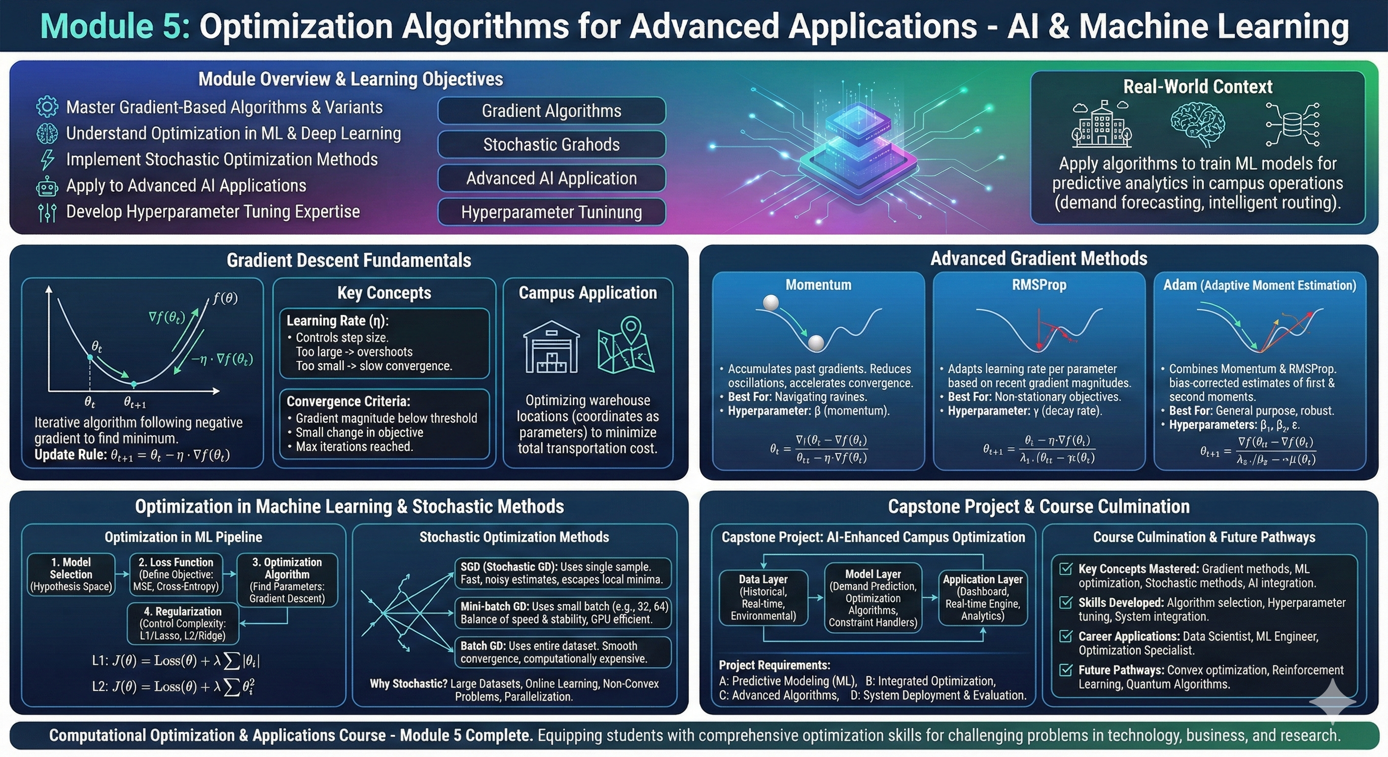
Apply optimization algorithms to train machine learning models for predictive analytics in campus operations, from demand forecasting to intelligent routing systems.
6.2 Gradient Descent Fundamentals
6.2.1 Theoretical Foundation
6.2.1.1 What is Gradient Descent?
Gradient Descent is an iterative optimization algorithm used to find the minimum of a function. By following the negative gradient of the function, it progressively moves toward the optimal solution.
6.2.1.2 Mathematical Formulation
Given a function \(f(\theta)\) we want to minimize:
Batch Gradient Descent: Uses entire dataset for each update
Stochastic Gradient Descent (SGD): Uses single sample per update
Mini-batch Gradient Descent: Uses small batches of data
6.2.1.4 Campus City Application
Optimizing warehouse locations by treating facility coordinates as parameters and total transportation cost as the objective function to minimize.
6.2.2 Sample Problem
Problem Statement: Minimize the quadratic function \(f(x) = x^2 - 4x + 4\) using gradient descent starting from \(x_0 = 0\), with learning rate \(\eta = 0.1\).
Solution Steps:
Gradient:\(\nabla f(x) = 2x - 4\)
Iteration 1:
Gradient at \(x_0 = 0\): \(2(0) - 4 = -4\)
Update: \(x_1 = 0 - 0.1(-4) = 0.4\)
Iteration 2:
Gradient at \(x_1 = 0.4\): \(2(0.4) - 4 = -3.2\)
Update: \(x_2 = 0.4 - 0.1(-3.2) = 0.72\)
Continue until convergence
Analytical minimum:\(x = 2\) (from setting gradient to zero)
Explain the intuition behind gradient descent: why does following the negative gradient lead to function minimization?
What is the effect of learning rate on gradient descent convergence? Provide examples of problems caused by too large and too small learning rates.
Calculate the first three iterations of gradient descent for \(f(x) = 3x^2 + 2x - 5\) starting from \(x_0 = 1\) with \(\eta = 0.05\).
How does gradient descent handle non-convex functions with multiple local minima?
Design a gradient descent approach for optimizing delivery routes in Campus City. What would be your parameters and objective function?
6.3 Advanced Gradient Methods
6.3.1 Theoretical Foundation
6.3.1.1 Limitations of Basic Gradient Descent
Slow convergence in flat regions
Oscillations in steep valleys
Sensitive to learning rate choice
Poor performance with ill-conditioned problems
As a solution, advanced gradient methods have been developed to address these issues by incorporating momentum, adaptive learning rates, and other techniques. Most of these methods are designed to accelerate convergence, improve stability, and handle the complexities of non-convex optimization landscapes commonly encountered in machine learning and deep learning applications. Popular methods include Momentum, Nesterov Accelerated Gradient (NAG), Adagrad, RMSProp, and Adam.
Poylak’s momentum method, introduced in 1964, is one of the earliest techniques to enhance gradient descent by adding a momentum term that helps accelerate convergence, especially in scenarios with high curvature or noisy gradients. The momentum term allows the optimization process to build up speed in directions with consistent gradients while dampening oscillations in directions with varying gradients. The update formula for Poylakis’s method is similar to the standard momentum method, where the velocity term is updated based on the current gradient and the previous velocity, and then used to update the parameters. This approach has been foundational in the development of more advanced optimization algorithms used in machine learning today. This method will solve the cold start problem. The update rules for Poylak’s momentum method can be expressed as:
A comparison of the gradient descent, momentum with EMA approach and the Poylak’s momentum method can be shown as follows:
Problem: Minimize \(f(x) = x^2 - 4x + 4\) starting from \(x_0 = 0\) with learning rate \(\eta = 0.1\) and momentum coefficient \(\beta = 0.9\).
Iteration
Standard GD
GD with EMA Momentum
Classical Polyak Momentum
0
0.0000
0.0000
0.0000
1
0.4000
0.0400
0.4000
2
0.7200
0.1152
1.0800
3
0.9760
0.2206
1.8760
4
1.1808
0.3510
2.6172
Nesterov Accelerated Gradient (NAG): Introduced by Yurii Nesterov in 1983, it has become a standard optimization technique in machine learning. Nesterov’s method looks ahead by calculating the gradient at the estimated future position: \[\begin{aligned}
v_t &= \beta v_{t-1} + (1 - \beta) \nabla f(\theta_t - \eta \beta v_{t-1}) \\
\theta_{t+1} &= \theta_t - \eta v_t
\end{aligned}
\] where the gradient is evaluated at the “look-ahead” position \(\theta_t - \eta \beta v_{t-1}\), allowing for more informed updates.
Provides a look-ahead mechanism
Often leads to faster convergence than standard momentum
Particularly effective in convex optimization problems
Can help escape local minima in non-convex problems
Reduces overshooting in steep regions
Commonly used in training deep neural networks for improved performance
6.3.1.2 Adaptive Learning Rate Methods
adaptive learning rate methods adjust the learning rate for each parameter based on the history of gradients, allowing for more efficient optimization, especially in scenarios with sparse gradients or varying curvature. Most common adaptive methods include Adagrad, RMSProp, and Adam, each with its own approach to modifying the learning rate dynamically during training.
Adagrad: Adapts learning rate for each parameter based on historical gradients. It divides the learning rate by the square root of the sum of squared gradients, which can lead to diminishing learning rates over time. The update formula is given by: \[
\theta_{t+1} = \theta_t - \frac{\eta}{\sqrt{G_t + \epsilon}} \nabla f(\theta_t)
\] Where \(G_t\) is the sum of squares of past gradients and \(\epsilon\) is a small constant to prevent division by zero. \[
G_t = \sum_{i=1}^t \nabla f(\theta_i)^2
\]
RMSProp: Adapts learning rate per parameter based on recent gradient magnitudes. Introduced in a 2012 Coursera lecture by Hinton, RMSProp aims to resolve Adagrad’s radically diminishing learning rates by using a moving average of squared gradients. Compare with Adagrad, RMSProp maintains a decaying average of past squared gradients, which allows it to continue learning even after many iterations. The update rules for RMSProp are: \[
\theta_{t+1} = \theta_t - \frac{\eta}{\sqrt{E[g^2]_t + \epsilon}} g_t
\] Where \(E[g^2]_t\) is the exponentially decaying average of past squared gradients, calculated as: \[E[g^2]_t = \gamma E[g^2]_{t-1} + (1 - \gamma) g_t^2\]
Adam (Adaptive Moment Estimation):
Adam is an optimization algorithm that combines the advantages of both Momentum and RMSProp. It computes adaptive learning rates for each parameter by maintaining running averages of both the gradients (first moment) and the squared gradients (second moment). Adam also includes bias-correction terms to account for the initialization of these averages. The update rules for Adam are as follows: \[\begin{aligned}
m_t &= \beta_1 m_{t-1} + (1 - \beta_1) g_t \\
v_t &= \beta_2 v_{t-1} + (1 - \beta_2) g_t^2 \\
\hat{m}_t &= \frac{m_t}{1 - \beta_1^t} \\
\hat{v}_t &= \frac{v_t}{1 - \beta_2^t} \\
\theta_{t+1} &= \theta_t - \frac{\eta}{\sqrt{\hat{v}_t} + \epsilon} \hat{m}_t
\end{aligned}
\]
where:
\(m_t\): First moment estimate (mean of gradients)
\(v_t\): Second moment estimate (uncentered variance of gradients)
\(\beta_1\): Exponential decay rate for the first moment estimates (commonly set to 0.9)
\(\beta_2\): Exponential decay rate for the second moment estimates (commonly set to 0.999)
\(\hat{m}_t\): Bias-corrected first moment estimate
\(\hat{v}_t\): Bias-corrected second moment estimate
\(\epsilon\): Small constant to prevent division by zero (commonly set to \(10^{-8}\))
Advantages of Adam:
Maintains exponentially decaying average of past gradients (first moment)
Maintains exponentially decaying average of past squared gradients (second moment)
Computes bias-corrected estimates
6.3.1.3 Mathematical Comparison
Method
Key Idea
Best For
Hyperparameters
Momentum
Accumulates past gradients
Navigating ravines
β (momentum)
NAG
Look-ahead gradient
Faster convergence
β (momentum)
RMSProp
Adaptive learning rates
Non-stationary objectives
γ (decay rate)
Adam
Combines momentum + RMSProp
General purpose
β₁, β₂, ε
6.3.2 Sample Problems
1. Problem statement: Compare the convergence of solutions of \(f(x)=x^2-4x+4\) using the Adagrad, RMSProp and adam optimizers starting from \(x_0=0\) with learning rate \(\eta=0.1\). Chose 4 iterations and show the results in a table. ( \(\gamma=0.9\), \(\beta_1=0.9\), \(\beta_2=0.99\) and \(\epsilon=10^{-8}\)).
import mathdef f_prime(x):"""Derivative of the objective function f(x) = x^2 - 4x + 4"""return2* x -4# Hyperparametersx_0 =0.0eta =0.1epsilon =1e-8iterations =4# AdaGrad Initializationx_ada = x_0G =0.0# RMSprop Initializationx_rms = x_0gamma =0.9E_g2 =0.0# Adam Initializationx_adam = x_0beta1 =0.9beta2 =0.99m =0.0v =0.0# Header for the tableprint(f"{'Iteration (t)':<15} | {'AdaGrad (x_t)':<15} | {'RMSprop (x_t)':<15} | {'Adam (x_t)':<15}")print("-"*68)print(f"{0:<15} | {x_0:<15.4f} | {x_0:<15.4f} | {x_0:<15.4f}")# Iteration Loopfor t inrange(1, iterations +1):# ------------------ AdaGrad Update ------------------ g_ada = f_prime(x_ada) G += g_ada**2 x_ada = x_ada - (eta / (math.sqrt(G) + epsilon)) * g_ada# ------------------ RMSprop Update ------------------ g_rms = f_prime(x_rms) E_g2 = gamma * E_g2 + (1- gamma) * g_rms**2 x_rms = x_rms - (eta / (math.sqrt(E_g2) + epsilon)) * g_rms# ------------------ Adam Update --------------------- g_adam = f_prime(x_adam) m = beta1 * m + (1- beta1) * g_adam v = beta2 * v + (1- beta2) * g_adam**2# Bias corrections for Adam m_hat = m / (1- beta1**t) v_hat = v / (1- beta2**t) x_adam = x_adam - (eta / (math.sqrt(v_hat) + epsilon)) * m_hat# Print rowprint(f"{t:<15} | {x_ada:<15.4f} | {x_rms:<15.4f} | {x_adam:<15.4f}")
Basic GD: May oscillate in the valley near \(x = 1\)
Momentum GD: Smoothens oscillations and converges faster
Key Insight: Momentum helps escape local flat regions and reduces zigzagging
Parameters:
Learning rate: \(\eta = 0.01\)
Momentum: \(\beta = 0.9\)
True minimum: Near \(x ≈ 0.85\)
6.3.3 Sample Problem
Problem Statement: A neural network for predicting campus facility demand has loss function with very different curvatures in different parameter directions (ill-conditioned). Which optimizer would you choose and why?
Solution:
Adam optimizer would be most suitable because:
Handles sparse gradients well
Adapts learning rates per parameter
Combines benefits of momentum and RMSProp
Generally robust to ill-conditioning
6.3.4 Review Questions
Explain how momentum helps gradient descent overcome the problem of oscillations in narrow valleys.
Compare RMSProp and Adam optimizers. When would you choose one over the other for campus demand prediction?
What is the “look-ahead” property of Nesterov Accelerated Gradient and how does it improve convergence?
Design an adaptive learning rate schedule for optimizing a campus energy consumption model. What factors would influence your schedule?
How do advanced gradient methods handle the trade-off between convergence speed and stability?
6.4 Optimization in Machine Learning
In previous sections, we focused on optimization algorithms in a general context. Now, we will explore how these optimization techniques are applied specifically in machine learning and deep learning contexts, where the objective is to minimize a loss function that measures the discrepancy between predicted and true values. Optimization in machine learning involves not only finding the best parameters for a model but also ensuring that the model generalizes well to unseen data, which introduces additional challenges such as overfitting and underfitting.
6.4.1 Theoretical Foundation
In machine learning, optimization is central to training models. The goal is to find the parameters that minimize a loss function, which quantifies the error between the model’s predictions and the actual data.
6.4.1.1 Optimization in ML Pipeline
A ML problem typically involves the following steps:
Model Selection: Choose a model architecture (e.g., linear regression, neural network).
Loss Function: Define a loss function that quantifies the error between predictions and true labels.
Optimization Algorithm: Choose an optimization algorithm to minimize the loss function.
Regularization: Add regularization terms to prevent overfitting and improve generalization.
6.4.1.2 Model Selection
Lets starts with the model selection. The choice of model architecture can significantly impact the optimization process. For example, linear models have convex loss landscapes, which guarantee that gradient descent will converge to a global minimum. In contrast, deep neural networks have non-convex loss landscapes with multiple local minima and saddle points, making optimization more challenging. The choice of model also influences the choice of optimization algorithm, as certain algorithms may be better suited for specific types of models or loss functions. Model selection should be guided by the complexity of the data, the amount of available training data, and the specific task at hand (e.g., regression vs. classification).
6.4.1.3 Loss Functions
The loss function is a critical component of the optimization process in machine learning, as it defines the objective that the optimization algorithm seeks to minimize. The choice of loss function depends on the type of problem being solved (e.g., regression, classification) and can significantly affect the convergence and performance of the model. The loss function should be chosen to reflect the specific goals of the model and the characteristics of the data. For instance, mean squared error is commonly used for regression tasks, while cross-entropy loss is typically used for classification tasks. The properties of the loss function, such as convexity and differentiability, also play a crucial role in determining the optimization landscape and the behavior of the optimization algorithm. Common loss functions include mean squared error, cross-entropy, and hinge loss, each with its own advantages and disadvantages depending on the context of the problem being addressed.
Common Loss Functions:
Mean Squared Error (MSE):\(\frac{1}{n} \sum (y_i - \hat{y}_i)^2\): Used for regression tasks, penalizes larger errors more heavily, and is sensitive to outliers. For example, if a dataset contains an outlier with a large error, the MSE will be significantly affected, leading to a model that may not generalize well to the majority of the data. In contrast, using a loss function like Huber loss can mitigate this issue by reducing the influence of outliers on the optimization process. Advantages of MSE include its simplicity and the fact that it provides a smooth gradient for optimization, which can lead to efficient convergence. However, its sensitivity to outliers can be a significant drawback in certain applications, such as when the data contains noise or extreme values that do not represent the underlying distribution well. Along with its advantages, MSE’s sensitivity to outliers can lead to skewed model performance, as the optimization process may focus on minimizing the error for outliers at the expense of fitting the majority of the data accurately. This can result in a model that performs poorly on unseen data, especially if the outliers are not representative of the true underlying patterns in the data. Therefore, while MSE is a widely used loss function for regression tasks, it is important to consider the characteristics of the dataset and the presence of outliers when choosing an appropriate loss function for optimization.
Mean Absolute Error (MAE):\(\frac{1}{n} \sum |y_i - \hat{y}_i|\): Also used for regression, less sensitive to outliers than MSE, and provides a linear penalty for errors. For instance, if a dataset contains an outlier with a large error, the MAE will be less affected compared to MSE, as it does not square the error term. This makes MAE a more robust choice in situations where the data may contain noise or extreme values that do not represent the underlying distribution well. However, MAE can lead to slower convergence during optimization due to its non-differentiability at zero, which can make it more challenging to optimize using gradient-based methods. Despite this drawback, MAE’s robustness to outliers can make it a preferable choice in certain regression tasks where the presence of outliers is a concern. Advantages of MAE include its simplicity and robustness to outliers, while its disadvantages include potential challenges in optimization due to non-differentiability and slower convergence compared to MSE. When choosing between MSE and MAE, it is important to consider the specific characteristics of the dataset and the goals of the modeling task, as well as the trade-offs between sensitivity to outliers and optimization efficiency. There are disadvantages to using MAE, such as its non-differentiability at zero, which can lead to challenges in optimization using gradient-based methods. This can result in slower convergence compared to MSE, especially in cases where the model predictions are close to the true values. Additionally, MAE does not provide a smooth gradient for optimization, which can make it more difficult for certain optimization algorithms to find the optimal parameters efficiently. Despite these drawbacks, MAE’s robustness to outliers can make it a preferable choice in certain regression tasks where the presence of outliers is a concern. When choosing between MSE and MAE, it is important to consider the specific characteristics of the dataset and the goals of the modeling task, as well as the trade-offs between sensitivity to outliers and optimization efficiency.
Cross-Entropy:\(-\sum y_i \log(\hat{y}_i)\): Used for classification tasks, measures the difference between true labels and predicted probabilities, and is effective for training models that output probabilities. For instance, in a binary classification problem, if the model predicts a probability of 0.9 for the positive class when the true label is 1, the cross-entropy loss will be low, indicating a good prediction. However, if the model predicts a probability of 0.1 for the positive class, the loss will be high, signaling a poor prediction. Advantages of cross-entropy loss include its ability to provide a smooth gradient for optimization and its suitability for classification tasks, particularly when the model outputs probabilities. However, one disadvantage of cross-entropy loss is that it can be sensitive to class imbalance, where one class is significantly more prevalent than the other. In such cases, the model may become biased towards the majority class, leading to poor performance on the minority class. To address this issue, techniques such as class weighting or using alternative loss functions like focal loss can be employed to improve model performance in imbalanced classification scenarios. When choosing a loss function for classification tasks, it is important to consider the specific characteristics of the dataset, including class distribution and the goals of the modeling task, as well as the trade-offs between optimization efficiency and sensitivity to class imbalance. Its major disadvantage is that it can be sensitive to class imbalance, where one class is significantly more prevalent than the other. In such cases, the model may become biased towards the majority class, leading to poor performance on the minority class. To address this issue, techniques such as class weighting or using alternative loss functions like focal loss can be employed to improve model performance in imbalanced classification scenarios. When choosing a loss function for classification tasks, it is important to consider the specific characteristics of the dataset, including class distribution and the goals of the modeling task, as well as the trade-offs between optimization efficiency and sensitivity to class imbalance.
Categorical Cross-Entropy:\(-\sum y_i \log(\hat{y}_i)\): Used for multi-class classification, generalizes cross-entropy to multiple classes, and is effective for training models that output class probabilities. For example, in a multi-class classification problem with three classes, if the model predicts probabilities of [0.7, 0.2, 0.1] for the true class being the first class (1), the categorical cross-entropy loss will be low, indicating a good prediction. However, if the model predicts probabilities of [0.1, 0.2, 0.7], the loss will be high, signaling a poor prediction. Advantages of categorical cross-entropy loss include its ability to provide a smooth gradient for optimization and its suitability for multi-class classification tasks, particularly when the model outputs class probabilities. However, one disadvantage of categorical cross-entropy loss is that it can be sensitive to class imbalance, where one class is significantly more prevalent than the others. In such cases, the model may become biased towards the majority class, leading to poor performance on minority classes. To address this issue, techniques such as class weighting or using alternative loss functions like focal loss can be employed to improve model performance in imbalanced multi-class classification scenarios. When choosing a loss function for multi-class classification tasks, it is important to consider the specific characteristics of the dataset, including class distribution and the goals of the modeling task, as well as the trade-offs between optimization efficiency and sensitivity to class imbalance.
Hinge Loss:\(\max(0, 1 - y_i \hat{y}_i)\): Used in support vector machines, encourages a margin between classes, and is non-differentiable at the margin. For example, if a data point is correctly classified with a margin greater than 1, the hinge loss will be zero, indicating no penalty. However, if a data point is misclassified or classified within the margin (i.e., \(y_i \hat{y}_i < 1\)), the hinge loss will be positive, penalizing the model for not maintaining the desired margin. Common applications of hinge loss include support vector machines (SVMs) for classification tasks, where the goal is to find a hyperplane that maximizes the margin between classes. Advantages of hinge loss include its ability to encourage a margin between classes and its suitability for SVMs, while its disadvantages include non-differentiability at the margin, which can make optimization more challenging. When using hinge loss, it is important to consider the specific characteristics of the dataset and the goals of the modeling task, as well as the trade-offs between optimization efficiency and the desire to maintain a margin between classes. Advantages of hinge loss include its ability to encourage a margin between classes and its suitability for SVMs, while its disadvantages include non-differentiability at the margin, which can make optimization more challenging. When using hinge loss, it is important to consider the specific characteristics of the dataset and the goals of the modeling task, as well as the trade-offs between optimization efficiency and the desire to maintain a margin between classes.
Properties of loss functions:
Three key properties of loss functions that influence optimization are:
Convexity affects optimization difficulty: convex functions guarantee global minima, while non-convex functions may have multiple local minima. A loss function is convex if its second derivative is non-negative for all inputs, which ensures that any local minimum is also a global minimum. Non-convex loss functions can lead to optimization challenges, as they may contain multiple local minima and saddle points, making it difficult for gradient-based methods to find the global minimum. Using the example of a simple quadratic loss function, we can see that it is convex because its second derivative is constant and positive. In contrast, a loss function with multiple peaks and valleys would be non-convex, posing challenges for optimization algorithms.
Mathematically, if \((\theta_1, \theta_2)\) are two points in the parameter space and \(\lambda \in [0, 1]\), a loss function \(L(\theta)\) is convex if: \[L(\lambda \theta_1 + (1 - \lambda) \theta_2) \leq \lambda L(\theta_1) + (1 - \lambda) L(\theta_2)\]
Differentiability determines gradient availability: differentiable loss functions allow for gradient-based optimization methods, while non-differentiable loss functions may require subgradient methods or other optimization techniques. For example, the hinge loss used in support vector machines is non-differentiable at the point where \(y_i \hat{y}_i = 1\), which necessitates the use of subgradient methods for optimization. In contrast, the mean squared error loss is differentiable everywhere, allowing for straightforward application of gradient descent.
Robustness to outliers influences performance: loss functions like Huber loss are designed to be less sensitive to outliers compared to MSE, which can be heavily influenced by extreme values. The Huber loss behaves like MSE for small residuals and like absolute error for large residuals, providing a balance between sensitivity and robustness. In contrast, the mean squared error can disproportionately penalize outliers, leading to skewed model performance. For instance, if a dataset contains outliers, using MSE as the loss function may result in a model that fits the outliers at the expense of overall performance, while Huber loss would mitigate this issue by reducing the influence of outliers on the optimization process.
6.4.2 Bias and Variance
Bias: Error from erroneous assumptions in the learning algorithm. High bias can cause underfitting, where the model is too simple to capture the underlying patterns in the data. For example, a linear regression model may have high bias when trying to fit a dataset with a non-linear relationship between the features and the target variable, leading to poor performance on both training and test data.
Variance: Error from sensitivity to small fluctuations in the training set. High variance can cause overfitting, where the model captures noise in the training data and fails to generalize to unseen data. For instance, a high-degree polynomial regression model may have high variance when fitting a dataset with limited samples, as it may capture noise and outliers in the training data, resulting in poor performance on test data.
Bias-Variance Trade-off
The bias-variance trade-off is a fundamental concept in machine learning that describes the relationship between bias and variance in model performance. As model complexity increases, bias tends to decrease while variance tends to increase. The optimal model complexity is achieved when the total error (sum of bias and variance) is minimized. For example, a simple linear model may have high bias but low variance, while a complex neural network may have low bias but high variance. The goal is to find a balance that minimizes total error and achieves good generalization to unseen data.
6.4.3 Overfitting and Underfitting
Overfitting: Model captures noise in training data, performs poorly on unseen data. It occurs when a model is too complex relative to the amount of training data, leading to a model that fits the training data very well but fails to generalize to new, unseen data. For example, a high-degree polynomial regression model may fit the training data perfectly but will likely perform poorly on test data due to its sensitivity to noise and outliers.
Underfitting: Model is too simple, fails to capture underlying patterns in data. It occurs when a model is not complex enough to capture the underlying structure of the data, resulting in poor performance on both the training and test datasets. For instance, a linear regression model may underfit a dataset that has a non-linear relationship between the features and the target variable, leading to high bias and poor predictive performance.
Methods to handle overfitting and underfitting:
Cross-validation: Evaluates model performance on unseen data to detect overfitting. By partitioning the dataset into training and validation sets, cross-validation allows for the assessment of how well a model generalizes to new data. For example, k-fold cross-validation involves dividing the dataset into k subsets, training the model on k-1 subsets, and validating it on the remaining subset. This process is repeated k times, with each subset serving as the validation set once, providing a more reliable estimate of model performance and helping to identify overfitting.
Regularization: Adds penalty to loss function to prevent overfitting. Regularization techniques, such as L1 and L2 regularization, introduce a penalty term to the loss function that discourages complex models by shrinking the coefficients of less important features towards zero. For instance, L1 regularization (Lasso) can lead to sparse models by driving some coefficients to exactly zero, effectively performing feature selection, while L2 regularization (Ridge) encourages smaller coefficients without necessarily eliminating any features, helping to prevent overfitting while maintaining all features in the model.
6.4.3.1 Regularization Techniques
Regularization adds a penalty to the loss function to prevent overfitting and improve generalization. It can be viewed as adding a constraint to the optimization problem, encouraging simpler models that are less likely to fit noise in the training data. Common regularization techniques include L1 (Lasso), L2 (Ridge), and Elastic Net, each with its own mathematical formulation and effects on the model parameters.
L1 Regularization (Lasso):
In L1 regularization, the penalty is proportional to the absolute value of the coefficients. The objective function with L1 regularization can be expressed as: \[
J(\theta) = \text{Loss}(\theta) + \lambda \sum |\theta_i|
\]
Adavantages of L1 Regularization:
Promotes sparsity: Encourages many coefficients to be exactly zero, leading to simpler models and feature selection.
Feature selection: By driving some coefficients to zero, L1 regularization effectively selects a subset of features, which can be particularly beneficial in high-dimensional datasets where many features may be irrelevant or redundant. This can lead to more interpretable models and improved generalization performance by reducing overfitting.
L2 Regularization (Ridge): L2 regularization adds a penalty proportional to the square of the coefficients. The objective function with L2 regularization is given by: \[
J(\theta) = \text{Loss}(\theta) + \lambda \sum \theta_i^2
\]
Advantages of L2 Regularization:
Prevents overfitting: Encourages smaller coefficients, which can help prevent overfitting by reducing model complexity and improving generalization to unseen data. By adding a penalty on the magnitude of the coefficients, L2 regularization discourages the model from fitting the noise in the training data, leading to better performance on test data.
Stabilizes optimization: L2 regularization can help stabilize the optimization process by preventing large updates to the coefficients, which can lead to more stable convergence and improved performance, especially in cases where the features are highly correlated.
Elastic Net: Elastic Net combines both L1 and L2 regularization, allowing for a balance between sparsity and coefficient shrinkage. The objective function for Elastic Net is: \[
J(\theta) = \text{Loss}(\theta) + \lambda_1 \sum |\theta_i| + \lambda_2 \sum \theta_i^2
\] Where \(\lambda_1\) and \(\lambda_2\) are the regularization parameters for L1 and L2 terms, respectively.
Advantages of Elastic Net:
Combines benefits of L1 and L2: Provides a balance between feature selection (L1) and coefficient shrinkage (L2), making it effective in scenarios with correlated features or when the number of features exceeds the number of samples.
Flexibility: By adjusting the regularization parameters, Elastic Net can be tailored to specific datasets and modeling needs, allowing for greater flexibility in controlling model complexity and improving generalization performance.
6.4.3.2 Neural Network Optimization
We have covered the basics of optimization in machine learning, but optimizing neural networks introduces additional challenges due to their non-convex loss landscapes and high-dimensional parameter spaces. Neural network optimization often requires specialized techniques to ensure effective training and convergence. In addition to the advanced gradient methods discussed earlier, there are several key considerations when optimizing neural networks:
Special considerations for deep learning:
Vanishing/Exploding Gradients: Gradients can become very small (vanishing) or very large (exploding) in deep networks, making training difficult. Solutions include using ReLU activation functions, batch normalization, and careful weight initialization.
Batch Normalization: Stabilizes training: normalizes layer inputs, allowing for higher learning rates and faster convergence. It also helps mitigate the vanishing gradient problem by maintaining a more stable distribution of activations throughout the network, which can lead to improved performance and faster training times.
Dropout: Regularization technique: randomly drops units during training to prevent overfitting and improve generalization. By randomly deactivating a subset of neurons during each training iteration, dropout forces the network to learn more robust features that are not reliant on specific neurons, thereby reducing the risk of overfitting and improving the model’s ability to generalize to unseen data. By introducing randomness into the training process, dropout can also help prevent co-adaptation of neurons, leading to a more resilient and effective model.Andrew Ng’s Deep Learning Specialization on Coursera provides an in-depth exploration of these techniques and their applications in optimizing neural networks for various tasks, including computer vision, natural language processing, and more. The formula suggested by Andrew Ng for dropout is: \[\text{Dropout}(x) = \frac{x \cdot \text{Bernoulli}(p)}{p}\]
Where \(x\) is the input to the dropout layer, \(\text{Bernoulli}(p)\) is a random variable that takes the value 1 with probability \(p\) and 0 with probability \(1-p\), and the division by \(p\) is used to maintain the expected value of the activations during training. This technique effectively prevents overfitting by randomly deactivating a fraction of the neurons during each training iteration, encouraging the network to learn more robust features that are not reliant on specific neurons. By introducing randomness into the training process, dropout can also help prevent co-adaptation of neurons, leading to a more resilient and effective model.
Weight Initialization: Proper weight initialization can help mitigate issues like vanishing/exploding gradients and improve convergence. Techniques include Xavier/Glorot initialization and He initialization, which are designed to maintain the variance of activations across layers, promoting stable training and faster convergence. For example, Xavier initialization is given by: \[W \sim \mathcal{U}\left(-\sqrt{\frac{6}{n_{in} + n_{out}}}, \sqrt{\frac{6}{n_{in} + n_{out}}}\right)\]
Where \(n_{in}\) and \(n_{out}\) are the number of input and output units in the layer, respectively. This initialization method helps maintain the variance of activations across layers, which can lead to improved convergence and performance during training. He initialization, on the other hand, is given by: \[W \sim \mathcal{N}\left(0, \sqrt{\frac{2}{n_{in}}}\right)\]
Where \(n_{in}\) is the number of input units in the layer. He initialization is particularly effective for layers with ReLU activation functions, as it helps mitigate the vanishing gradient problem by maintaining a more stable distribution of activations throughout the network, leading to improved performance and faster training times.
6.4.4 Sample Problem
Problem Statement: Train a linear regression model for predicting campus facility demand with features: day_of_week, temperature, special_event. Use gradient descent with L2 regularization.
Mathematical Formulation: Based on the problem statement, we can formulate the optimization problem for training a linear regression model with L2 regularization as follows: \[
J(\theta) = \frac{1}{2m} \sum_{i=1}^m (h_\theta(x^{(i)}) - y^{(i)})^2 + \frac{\lambda}{2m} \sum_{j=1}^n \theta_j^2
\] Where:
Gradient with Regularization: The gradient of the cost function with respect to the parameters \(\theta_j\) for \(j \geq 1\) can be derived as follows: \[
\frac{\partial J}{\partial \theta_j} = \frac{1}{m} \sum_{i=1}^m (h_\theta(x^{(i)}) - y^{(i)}) x_j^{(i)} + \frac{\lambda}{m} \theta_j \quad \text{for } j \geq 1
\]
C:\Users\SIJUKSWAMY\AppData\Local\Temp\ipykernel_50068\3733090581.py:5: RuntimeWarning:

overflow encountered in square

C:\Users\SIJUKSWAMY\AppData\Local\Temp\ipykernel_50068\3733090581.py:14: RuntimeWarning:

invalid value encountered in subtract
6.4.5 Sample Problem
Problem Statement: A campus energy consumption prediction model uses neural network with 3 hidden layers. During training, gradients become extremely small in early layers. Identify the problem and solution.
Analysis: Given the problem statement, the issue of gradients becoming extremely small in early layers of a neural network is commonly referred to as the “vanishing gradient problem.” This problem occurs when the gradients of the loss function with respect to the parameters in the early layers become very small, effectively preventing those layers from learning and updating their weights during training.
Problem: Vanishing Gradient Problem
Causes: Deep network, activation functions like sigmoid
Solutions: There are several techniques to address the vanishing gradient problem in deep neural networks:
Use ReLU activation functions: ReLU (Rectified Linear Unit) activation functions help mitigate the vanishing gradient problem by allowing gradients to flow more effectively through the network. Unlike sigmoid or tanh activations, which can saturate and lead to small gradients, ReLU does not saturate for positive inputs, allowing for larger gradients and improved learning in deeper layers.
Implement batch normalization: Batch normalization can help stabilize the training process and mitigate the vanishing gradient problem by normalizing the inputs to each layer. This technique allows for higher learning rates and faster convergence, as it helps maintain a more stable distribution of activations throughout the network, which can lead to improved performance and faster training times.
Use residual connections: Residual connections, as introduced in ResNet architectures, allow for the flow of gradients directly through skip connections, bypassing one or more layers. This helps mitigate the vanishing gradient problem by providing an alternative path for gradients to flow, enabling deeper networks to be trained effectively.
Proper weight initialization: Using appropriate weight initialization techniques, such as Xavier or He initialization, can help maintain the variance of activations across layers, which can mitigate the vanishing gradient problem and promote stable training and faster convergence.
Selecting the appropriate solution depends on the specific architecture and requirements of the neural network being trained, as well as the nature of the dataset and the problem being addressed.
6.4.6 Review Questions
Explain how regularization prevents overfitting in machine learning optimization from an optimization theory perspective.
Compare L1 and L2 regularization. When would you choose each for campus facility demand prediction?
What is the vanishing gradient problem in deep learning and how do modern optimizers address it?
Design a loss function for optimizing campus shuttle bus schedules that considers both operational costs and passenger wait times.
How does mini-batch gradient descent balance the trade-off between computational efficiency and convergence stability?
6.5 Stochastic Optimization Methods
Stochastic optimization methods are essential for training machine learning models on large datasets, where computing the full gradient can be computationally expensive. These methods use random subsets of data to estimate the gradient, allowing for faster iterations and the ability to escape local minima in non-convex optimization problems.
6.5.1 Theoretical Foundation
Computing the full gradient of the loss function with respect to the model parameters can be computationally expensive, especially for large datasets. Stochastic optimization methods address this issue by using random subsets of data (mini-batches) to estimate the gradient, allowing for faster iterations and the ability to escape local minima in non-convex optimization problems. Convergence analysis of stochastic optimization methods often involves understanding the trade-offs between bias and variance in the gradient estimates, as well as the impact of learning rate schedules on convergence rates.
6.5.1.1 Why Stochastic Optimization?
Main reasons for using stochastic optimization methods include:
Large Datasets: Full gradient computation is expensive. Stochastic methods provide faster updates by using mini-batches. For example, in a dataset with 1 million samples, computing the full gradient would require processing all 1 million samples for each update, which can be computationally prohibitive. In contrast, using mini-batches of size 64 allows for much faster updates while still providing a reasonable estimate of the gradient.
Online Learning: Stochastic methods can update models in real-time as new data arrives, making them suitable for dynamic environments. For instance, in a campus energy management system, new sensor data may be continuously generated. Stochastic optimization allows the model to be updated in real-time, enabling it to adapt to changing conditions and improve predictions without needing to retrain on the entire dataset.
Non-Convex Problems: Stochastic methods can escape local minima, which is crucial for training deep neural networks. In non-convex optimization problems, such as training deep neural networks, the loss landscape can contain many local minima and saddle points. Stochastic optimization methods, by introducing noise into the gradient estimates, can help the optimization process escape these local minima and saddle points, leading to better convergence to a global minimum or a more optimal solution.
Parallelization: Stochastic methods can be parallelized across multiple processors or GPUs, improving training speed. For example, mini-batch gradient descent can be easily parallelized by distributing the computation of gradients across multiple GPUs, allowing for faster training times and the ability to handle larger models and datasets.
6.5.1.2 Stochastic Gradient Descent (SGD)
We already covered the basics of stochastic gradient descent (SGD) in previous modules, but let’s briefly review it here in the context of stochastic optimization methods. SGD is a simple yet powerful optimization algorithm that updates model parameters using the gradient of the loss function with respect to a single training example (or a mini-batch of examples) at each iteration. The update rule for SGD can be expressed as follows:
Algorithm: For each epoch, for each training example \((x^{(i)}, y^{(i)})\):
Noisy gradient estimates: Each update is based on a single example, leading to high variance in the updates. This can cause the optimization process to be noisy and may lead to slower convergence compared to batch gradient descent. However, this noise can also help the optimization process escape local minima in non-convex problems, which is a significant advantage of SGD over batch gradient descent.
Faster per iteration: Each update is computationally cheaper than batch gradient descent, allowing for faster iterations. This can lead to quicker progress in the early stages of training, especially when dealing with large datasets.
May not converge to exact minimum: Due to the noise in the updates, SGD may not converge to the exact minimum of the loss function, but it can get close enough for practical purposes. The convergence behavior of SGD can be influenced by factors such as the learning rate and the choice of mini-batch size.
Can escape local minima in non-convex problems: The noise in the gradient estimates can help the optimization process escape local minima and saddle points, which is particularly beneficial when training deep neural networks.
# Example implementation of SGDimport numpy as npdef sgd(X, y, theta, alpha, iterations): m =len(y)for i inrange(iterations):for j inrange(m):# Randomly select a training example idx = np.random.randint(m) x_i = X[idx] y_i = y[idx]# Compute the gradient gradient = (x_i.dot(theta) - y_i) * x_i# Update parameters theta -= alpha * gradientreturn theta## sample usageX = np.array([[1, 0], [1, 1], [2, 0], [2, 1]]) # Add intercept termy = np.array([1, 2, 3, 4])theta = np.zeros(X.shape[1])alpha =0.01iterations =1000theta = sgd(X, y, theta, alpha, iterations)print("Optimized parameters:", theta)
Optimized parameters: [1.47484672 0.79455867]
6.5.1.3 Mini-batch Gradient Descent
Mini-batch gradient descent is a compromise between batch gradient descent and stochastic gradient descent. It updates model parameters using the average gradient computed from a small random subset of the training data (mini-batch) at each iteration. The update rule for mini-batch gradient descent can be expressed as follows:
Update Rule:\[
\theta := \theta - \eta \nabla_\theta J(\theta; x^{(i:i+n)}, y^{(i:i+n)})
\] Where batch size \(n\) is typically 32, 64, or 128.
Advantages of mini-batch gradient descent include:
Reduces variance compared to SGD: By using a mini-batch of examples to compute the gradient, mini-batch gradient descent provides a more stable and accurate estimate of the true gradient compared to SGD, which can lead to faster convergence and improved performance.
Hardware efficient (GPU parallelization): Mini-batch gradient descent can take advantage of parallel processing capabilities of modern hardware, such as GPUs, to compute gradients for multiple examples simultaneously, leading to faster training times. For example, using a mini-batch size of 64 allows for efficient computation of gradients on a GPU, as it can process multiple examples in parallel, while still providing a reasonable estimate of the gradient for updating the model parameters.
More stable convergence than pure SGD: The use of mini-batches helps to smooth out the noise in the gradient estimates, leading to more stable convergence compared to pure SGD, which can be highly noisy due to its reliance on single examples for updates. This stability can result in faster convergence and improved performance, especially when training deep neural networks on large datasets.
6.5.1.4 Advanced Stochastic Methods
In addition to basic SGD and mini-batch gradient descent, there are several advanced stochastic optimization methods that have been developed to improve convergence and performance in training machine learning models. These methods often incorporate techniques such as momentum, adaptive learning rates, and variance reduction to enhance the optimization process. Some of the most popular advanced stochastic optimization methods include:
SGD with Momentum: Incorporates a velocity term to accelerate convergence and reduce oscillations. The update rule for SGD with momentum can be expressed as follows: \[v := \beta v + (1 - \beta) \nabla_\theta J(\theta; x^{(i)}, y^{(i)})\]\[\theta := \theta - \eta v\] Where \(\beta\) is the momentum parameter, typically set to 0.9. This method helps to smooth out the updates and can lead to faster convergence, especially in scenarios where the loss landscape has narrow valleys or plateaus.
# Example implementation of SGD with Momentumdef sgd_momentum(X, y, theta, alpha, beta, iterations): m =len(y) v = np.zeros_like(theta)for i inrange(iterations):for j inrange(m): idx = np.random.randint(m) x_i = X[idx] y_i = y[idx] gradient = (x_i.dot(theta) - y_i) * x_i v = beta * v + (1- beta) * gradient theta -= alpha * vreturn theta # example usage X = np.array([[1, 0], [1, 1], [2, 0], [2, 1]]) # Add intercept termy = np.array([1, 2, 3, 4])theta = np.zeros(X.shape[1])alpha =0.01beta =0.9iterations =1000theta = sgd_momentum(X, y, theta, alpha, beta, iterations)print("Optimized parameters:", theta)
Optimized parameters: [1.4714003 0.83852972]
Adam for Stochastic Optimization: Combines momentum and adaptive learning rates for efficient optimization. The update rule for Adam can be expressed as follows: \[m := \beta_1 m + (1 - \beta_1) \nabla_\theta J(\theta; x^{(i)}, y^{(i)})\]\[v := \beta_2 v + (1 - \beta_2) (\nabla_\theta J(\theta; x^{(i)}, y^{(i)}))^2\]\[\hat{m} := \frac{m}{1 - \beta_1^t}\]\[\hat{v} := \frac{v}{1 - \beta_2^t}\]
where \(\beta_1\) and \(\beta_2\) are the decay rates for the moment estimates, typically set to 0.9 and 0.999, respectively. Adam is widely used in training deep neural networks due to its efficiency and effectiveness in handling sparse gradients and non-stationary objectives.
Learning Rate Scheduling: Adjusting the learning rate during training can improve convergence. Common schedules include:
Step decay: Reduce learning rate by a factor every few epochs. For example, reducing the learning rate by a factor of 0.1 every 10 epochs can help the optimization process converge more effectively as it allows for larger updates in the early stages of training and smaller, more fine-tuned updates as training progresses.
Exponential decay: Reduce learning rate exponentially over time. This can be expressed mathematically as:
\[\eta_t = \eta_0 \cdot e^{-\lambda t}\]
Where \(\eta_0\) is the initial learning rate, \(\lambda\) is the decay rate, and \(t\) is the current epoch or iteration. Exponential decay allows for a smooth and continuous reduction in the learning rate, which can help improve convergence and prevent overshooting as training progresses.
Cosine annealing: Reduce learning rate following a cosine curve, which can help escape local minima. The learning rate can be defined as:
Where \(\eta_{min}\) and \(\eta_{max}\) are the minimum and maximum learning rates, \(t\) is the current epoch or iteration, and \(T\) is the total number of epochs or iterations. Cosine annealing allows for a gradual reduction in the learning rate that follows a cosine curve, which can help the optimization process escape local minima and improve convergence, especially in non-convex optimization problems.
Warm restarts: Periodically reset learning rate to escape local minima. This can be implemented by resetting the learning rate to its initial value after a certain number of epochs or iterations, allowing the optimization process to escape local minima and potentially find better solutions. For example, resetting the learning rate every 10 epochs can help the optimization process explore different regions of the loss landscape and improve convergence.
6.5.1.5 Convergence Analysis
A general convergence analysis of stochastic optimization methods involves understanding the conditions under which these methods converge to a solution and the rates at which they do so. Theoretical guarantees for convergence often depend on assumptions about the loss function, such as convexity, smoothness, and the presence of noise in the gradient estimates.
Theoretical Guarantees:
The theoretical guarantees for convergence of stochastic optimization methods can be summarized as follows:
SGD converges to stationary point for non-convex functions: Under certain conditions, such as a diminishing learning rate and bounded gradients, stochastic gradient descent can be shown to converge to a stationary point of the loss function, even in non-convex optimization problems. This means that while SGD may not guarantee convergence to a global minimum, it can still find a point where the gradient is zero, which may correspond to a local minimum or saddle point.
Convergence rate: For convex loss functions, stochastic optimization methods like SGD can achieve a convergence rate of \(O(1/\sqrt{T})\), where \(T\) is the number of iterations. This means that the expected suboptimality of the solution decreases at a rate proportional to the inverse square root of the number of iterations, which is slower than the linear convergence rate of batch gradient descent but still provides a guarantee of improvement over time.
Mini-batch: Using mini-batches can improve convergence rates by reducing variance in gradient estimates, leading to faster convergence compared to pure SGD. The convergence rate of mini-batch gradient descent can be improved to \(O(1/T)\) under certain conditions, such as when the loss function is strongly convex and smooth. This improvement is due to the reduced variance in the gradient estimates provided by mini-batches, which allows for more stable updates and faster convergence compared to pure SGD.
6.5.2 Sample Problem
Problem Statement: Compare convergence behavior of batch GD, SGD, and mini-batch GD for optimizing a logistic regression model on campus facility usage data with 10,000 samples.
Analysis: From the problem statement, we can analyze the convergence behavior of batch gradient descent (GD), stochastic gradient descent (SGD), and mini-batch gradient descent (mini-batch GD) for optimizing a logistic regression model on campus facility usage data with 10,000 samples.
Batch GD: 10,000 computations per update, stable updates, but can get stuck in local minima. Batch gradient descent computes the gradient of the loss function with respect to the model parameters using the entire dataset of 10,000 samples for each update. This results in stable and accurate updates to the model parameters, as it uses the full information from the dataset. However, batch GD can be computationally expensive and may get stuck in local minima, especially in non-convex optimization problems like logistic regression on large datasets. The convergence of batch GD can be slow, particularly when dealing with large datasets, as it requires processing all samples for each update.
SGD: 1 computation per update, noisy updates, can escape local minima. Stochastic gradient descent computes the gradient using a single randomly selected sample from the dataset for each update. This results in noisy updates to the model parameters, as it relies on a single data point for each update, which can lead to high variance in the updates. However, this noise can also help SGD escape local minima in non-convex optimization problems, potentially leading to better convergence to a global minimum. The convergence of SGD can be faster in the early stages of training due to its ability to make quick updates, but it may require more iterations to converge compared to batch GD due to the noise in the updates.
Mini-batch (B=64): 64 computations per update, more stable than SGD, faster convergence than batch GD. Mini-batch gradient descent computes the gradient using a small random subset of the dataset (mini-batch) for each update. With a mini-batch size of 64, it provides a more stable and accurate estimate of the true gradient compared to SGD, while still being computationally efficient compared to batch GD. This can lead to faster convergence, especially when training deep neural networks on large datasets. The use of mini-batches helps to smooth out the noise in the gradient estimates, leading to more stable convergence compared to pure SGD, which can be highly noisy due to its reliance on single examples for updates.
Trade-offs: The main trade-offs between these methods include:
Computational cost per epoch: Batch GD is the most expensive, while SGD is the least expensive. Mini-batch GD falls in between, providing a balance between computational efficiency and convergence stability.
Convergence speed: SGD can converge faster in the early stages of training, while batch GD may take longer to converge due to its reliance on the entire dataset for each update. Mini-batch GD can provide faster convergence than batch GD while maintaining more stability than SGD.
Final solution quality: Batch GD may converge to a better local minimum due to its stable updates, while SGD may converge to a worse solution due to its noisy updates. Mini-batch GD can provide a good balance, potentially leading to better convergence than SGD while being more computationally efficient than batch GD.
Memory requirements: Batch GD requires more memory to store the entire dataset for each update, while SGD and mini-batch GD require less memory as they only need to store a single sample or a small subset of samples for each update.
6.5.3 Sample Problem
Problem Statement: Design a learning rate schedule for training a neural network on campus energy data that shows seasonal patterns.
Solution:
Cosine Annealing with Warm Restarts:
Start with relatively high learning rate
Gradually decrease following cosine curve
Periodically restart to escape local minima
Align restarts with seasonal transitions
Justification: Seasonal patterns create shifting data distributions, making warm restarts beneficial.
6.5.4 Review Questions
Explain why stochastic gradient descent can help escape local minima in non-convex optimization problems.
What is the optimal batch size for mini-batch gradient descent and how does it depend on problem characteristics?
Compare the convergence rates of SGD, mini-batch GD, and batch GD. When would you choose each method?
Design a distributed optimization strategy for training a campus-wide prediction model using stochastic methods.
How does learning rate scheduling improve stochastic optimization, particularly for non-stationary campus data?
6.6 Example- Implementation of concepts learned in Module 5 in the iris classification problem using Tensorflow and Keras
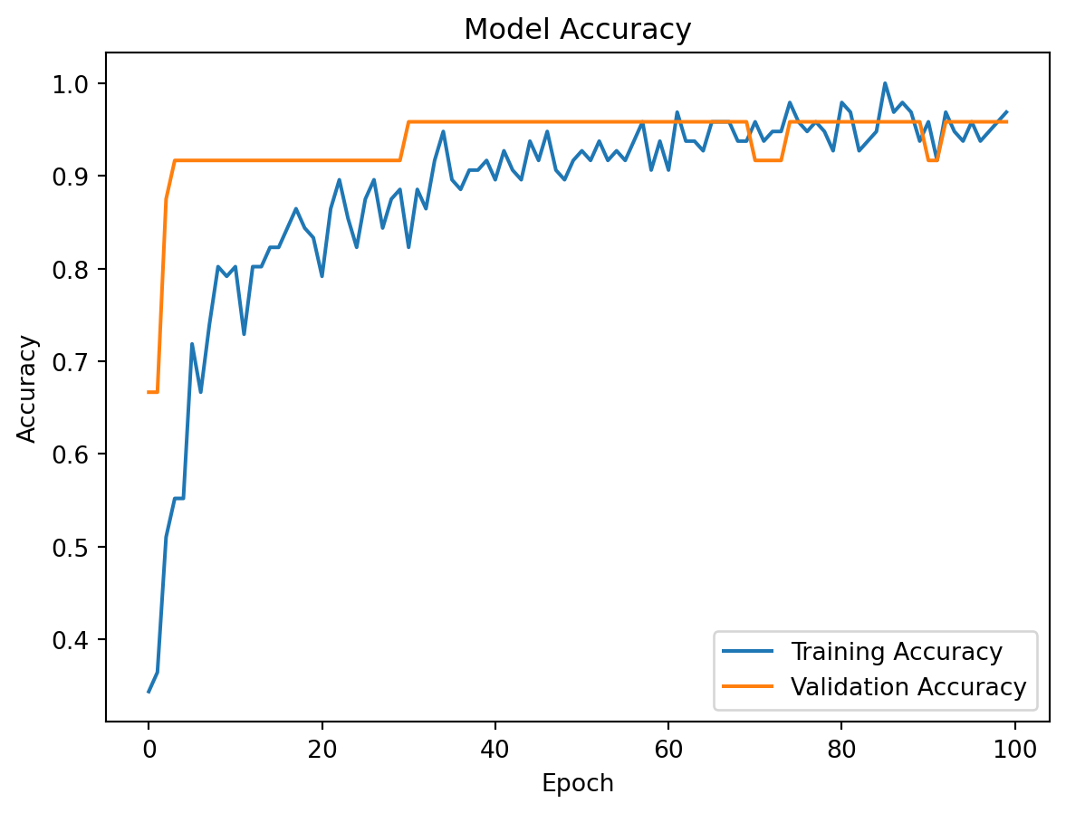
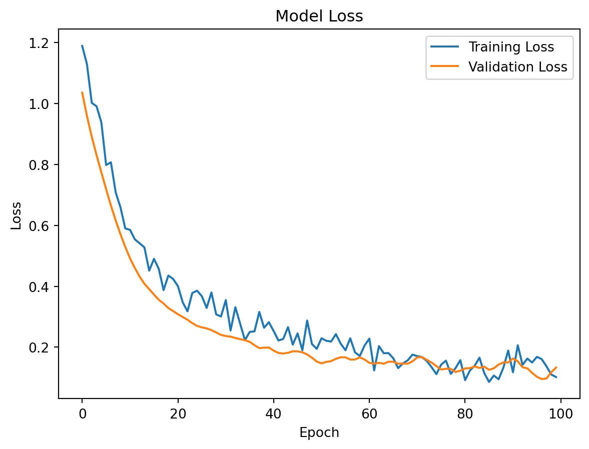
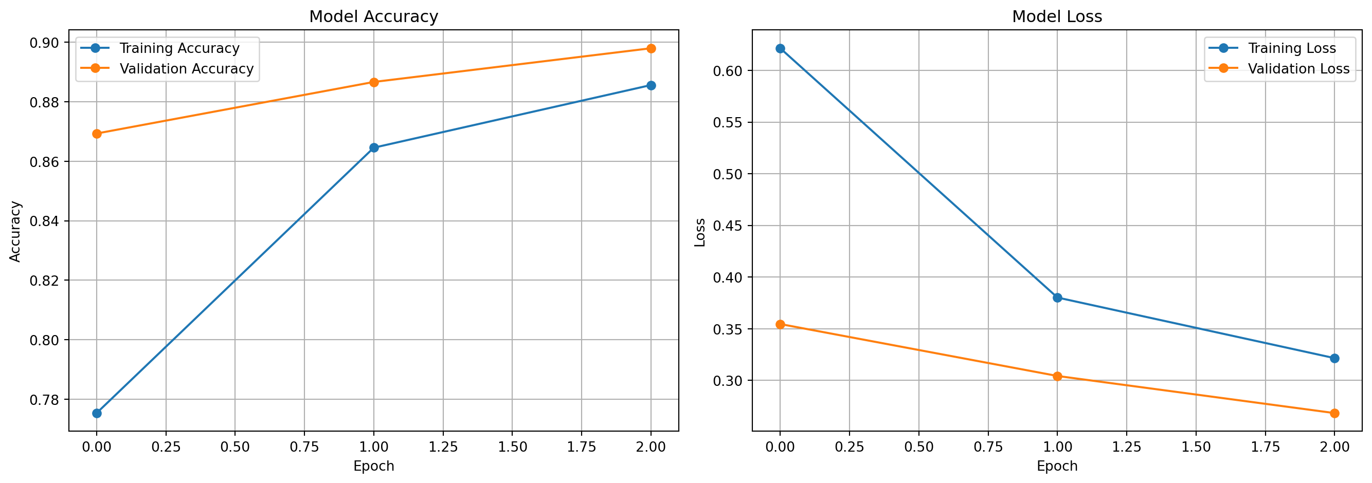
import tensorflow as tffrom tensorflow import kerasfrom sklearn.datasets import load_irisfrom sklearn.model_selection import train_test_splitfrom sklearn.metrics import accuracy_score,confusion_matrix, classification_report from sklearn.preprocessing import StandardScalerimport numpy as np# Load the iris datasetiris = load_iris()X = iris.datay = iris.target# Preprocess the datascaler = StandardScaler()X_scaled = scaler.fit_transform(X)# Split the data into training and testing setsX_train, X_test, y_train, y_test = train_test_split(X_scaled, y, test_size=0.2, random_state=42)# Build the neural network modelmodel = keras.Sequential([ keras.layers.Dense(64, activation='relu', input_shape=(X_train.shape[1],)), keras.layers.Dropout(0.5), keras.layers.Dense(64, activation='relu'), keras.layers.Dropout(0.5), keras.layers.Dense(3, activation='softmax')]) # Compile the model with Adam optimizer and categorical cross-entropy lossmodel.compile(optimizer='adam', loss='sparse_categorical_crossentropy', metrics=['accuracy'])# Train the modelhistory = model.fit(X_train, y_train, epochs=100, batch_size=16, validation_split=0.2,verbose=0)# Evaluate the model on the test set test_loss, test_acc = model.evaluate(X_test, y_test)print(f'Test accuracy: {test_acc:.4f}')print("Classification Report:")y_pred = np.argmax(model.predict(X_test), axis=1) print(classification_report(y_test, y_pred))#confusion matrixprint("Confusion Matrix:")print(confusion_matrix(y_test, y_pred))# false positives, false negatives, true positives, true negatives# For multi-class, you might want per-class metricscm = confusion_matrix(y_test, y_pred)# Get per-class metricsfor i inrange(len(cm)): tp = cm[i, i] fp = cm[:, i].sum() - tp fn = cm[i, :].sum() - tp tn = cm.sum() - (tp + fp + fn) precision = tp / (tp + fp) if (tp + fp) >0else0 recall = tp / (tp + fn) if (tp + fn) >0else0 f1 =2* (precision * recall) / (precision + recall) if (precision + recall) >0else0print(f"Class {i}: Precision={precision:.3f}, Recall={recall:.3f}, F1={f1:.3f}")# tru positives, true negatives, false positives, false negativesprint(f'True Positives: {tp}')print(f'True Negatives: {tn}')print(f'False Positives: {fp}')print(f'False Negatives: {fn}')# tru positive rate (sensitivity) and true negative rate (specificity)tpr = tp / (tp + fn) if (tp + fn) >0else0tnr = tn / (tn + fp) if (tn + fp) >0else0print(f'True Positive Rate (Sensitivity): {tpr:.4f}')print(f'True Negative Rate (Specificity): {tnr:.4f}')# Region of convergence plotimport matplotlib.pyplot as plt plt.plot(history.history['accuracy'], label='Training Accuracy')plt.plot(history.history['val_accuracy'], label='Validation Accuracy')plt.title('Model Accuracy')plt.xlabel('Epoch')plt.ylabel('Accuracy')plt.legend()plt.show()# Loss curve plot- training and validation loss curves to visualize convergence and potential overfittingplt.plot(history.history['loss'], label='Training Loss')plt.plot(history.history['val_loss'], label='Validation Loss')plt.title('Model Loss')plt.xlabel('Epoch') plt.ylabel('Loss')plt.legend()plt.show()
C:\Users\SIJUKSWAMY\AppData\Local\Programs\Python\Python312\Lib\site-packages\keras\src\layers\core\dense.py:87: UserWarning:

Do not pass an `input_shape`/`input_dim` argument to a layer. When using Sequential models, prefer using an `Input(shape)` object as the first layer in the model instead.
Statistical conclusion: The model achieves high accuracy on the test set, with a classification report showing strong precision, recall, and F1-score across all classes. The confusion matrix indicates that the model is effectively distinguishing between the three iris species, with minimal misclassifications. The training and validation curves suggest good convergence without significant overfitting, demonstrating the effectiveness of the optimization techniques applied in this module.
Major problems with the implementation: The model may require tuning of hyperparameters such as learning rate, batch size, and the number of epochs to achieve optimal performance. Additionally, the use of dropout layers may lead to underfitting if not properly balanced with the model architecture and training data. Finally, the small dataset size may limit the generalizability of the model, and further validation on larger datasets would be necessary to confirm its robustness.
Statistical issues with this loss function: The use of categorical cross-entropy loss is appropriate for multi-class classification problems like the iris dataset. However, if the dataset is imbalanced, this loss function may not adequately penalize misclassifications of minority classes, leading to biased predictions. In such cases, alternative loss functions or techniques such as class weighting or oversampling may be necessary to address class imbalance and improve model performance.
Issues with optimization of average loss: The optimization of average loss may not always lead to the best generalization performance, especially if the dataset contains outliers or is imbalanced. In such cases, the model may overfit to the majority class or be influenced by outliers, resulting in suboptimal performance on unseen data. To mitigate this issue, techniques such as robust loss functions, regularization, or data augmentation can be employed to improve the model’s ability to generalize and perform well on a wider range of inputs.
Truth of pixel-wise error minimization: Pixel-wise error minimization may not always lead to the best perceptual quality in image-related tasks, as it focuses on minimizing the average error across all pixels rather than considering the overall structure and context of the image. This can result in blurry or unrealistic outputs, especially in tasks such as image generation or super-resolution. To address this issue, alternative loss functions that consider perceptual quality, such as adversarial loss or perceptual loss, can be used to improve the visual quality of the generated images. In this context, it is a classification problem rather than an image generation task, so pixel-wise error minimization is not directly applicable. However, the choice of loss function and optimization strategy can still impact the model’s ability to generalize and perform well on unseen data, as discussed in the previous points. The real mathematics in the categorical cross-entropy loss function is based on the concept of maximum likelihood estimation, where the model is trained to maximize the likelihood of the observed data given the model parameters. This involves minimizing the negative log-likelihood, which is equivalent to minimizing the categorical cross-entropy loss in multi-class classification problems. The optimization process involves adjusting the model parameters to minimize this loss function, which can be achieved using various optimization algorithms such as SGD, Adam, or RMSProp, as discussed in this module. The categorical cross entropy measures the dissimilarity between the predicted probability distribution and the true distribution (one-hot encoded labels) for multi-class classification problems. It is defined as: \[L = -\sum_{i=1}^{N} \sum_{j=1}^{C} y_{ij} \log(p_{ij})\]
Where \(N\) is the number of samples, \(C\) is the number of classes, \(y_{ij}\) is the true label (1 if sample \(i\) belongs to class \(j\), 0 otherwise), and \(p_{ij}\) is the predicted probability that sample \(i\) belongs to class \(j\). The optimization process involves minimizing this loss function with respect to the model parameters, which can be achieved using various optimization algorithms such as SGD, Adam, or RMSProp, as discussed in this module. The choice of optimization algorithm and hyperparameters can significantly impact the convergence and performance of the model on the given dataset. This optimization uses the properties of the loss function, such as its smoothness and convexity, to guide the search for optimal parameters. The optimization process iteratively updates the model parameters in the direction that minimizes the loss function, ultimately leading to a model that can effectively classify the iris dataset with high accuracy and generalization performance.
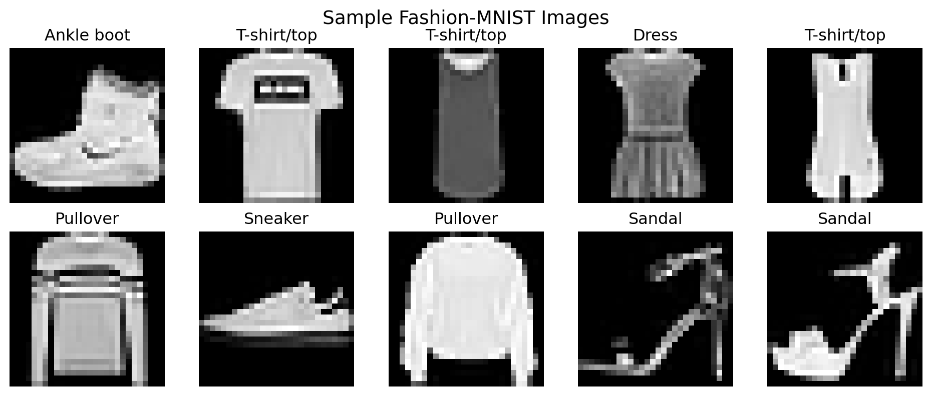
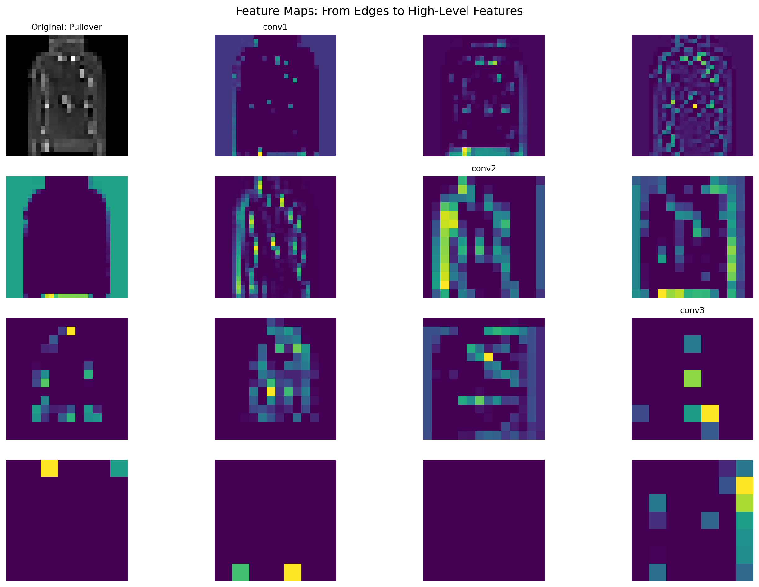
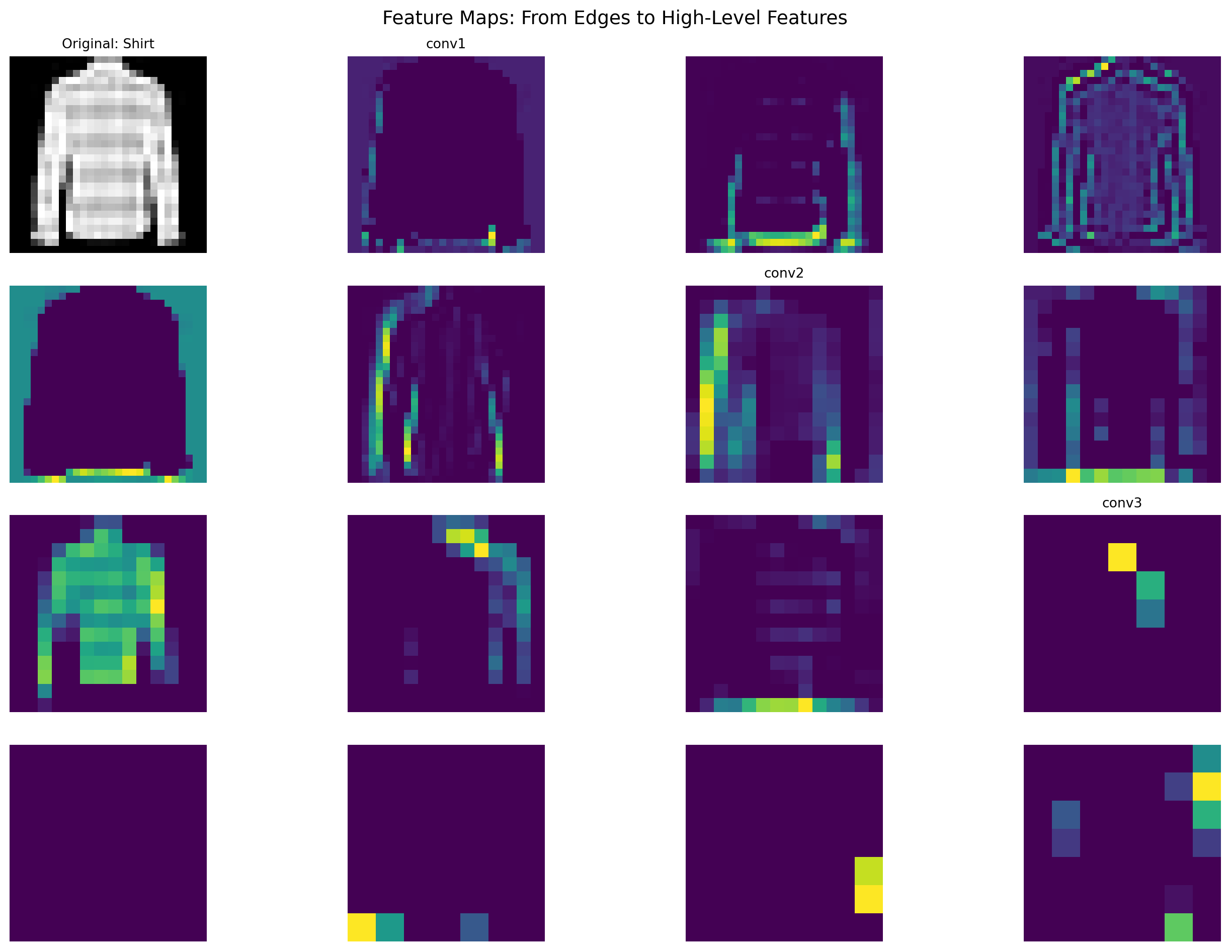
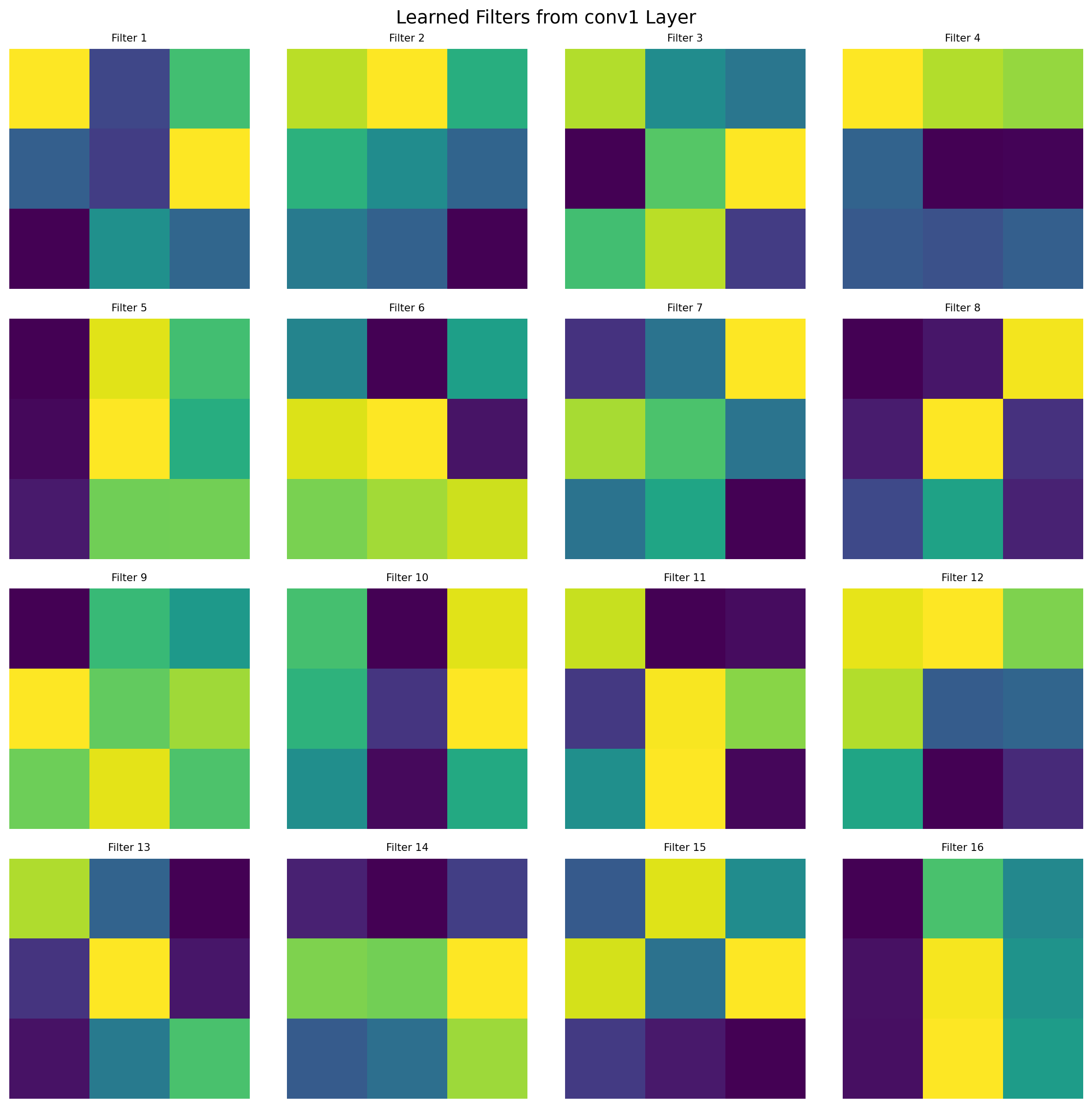
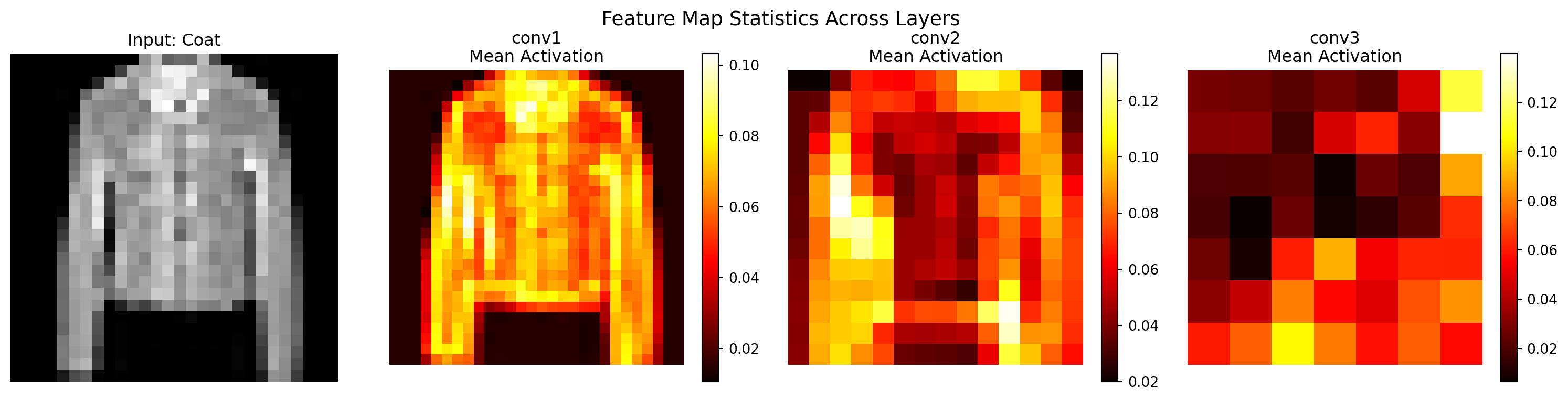
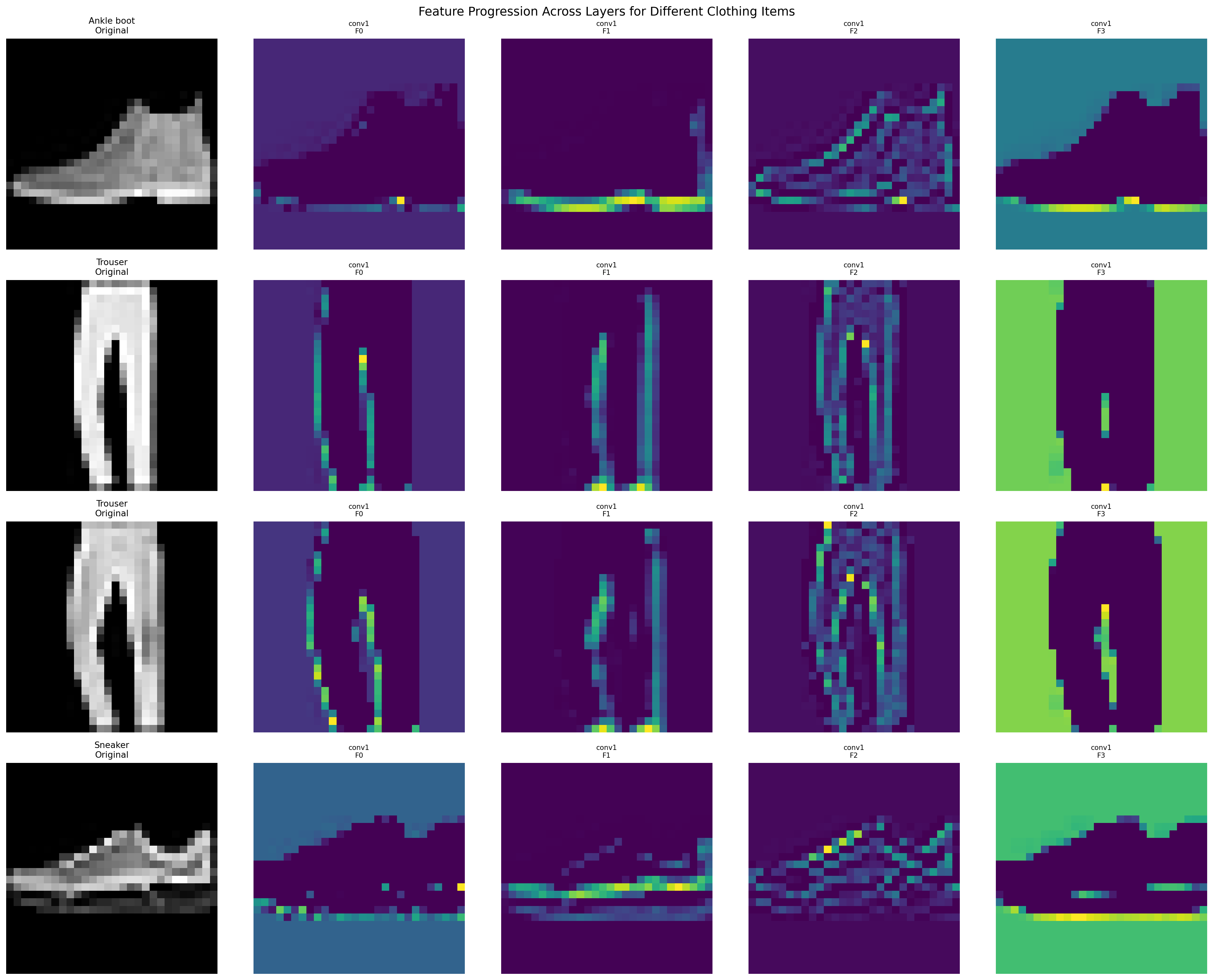
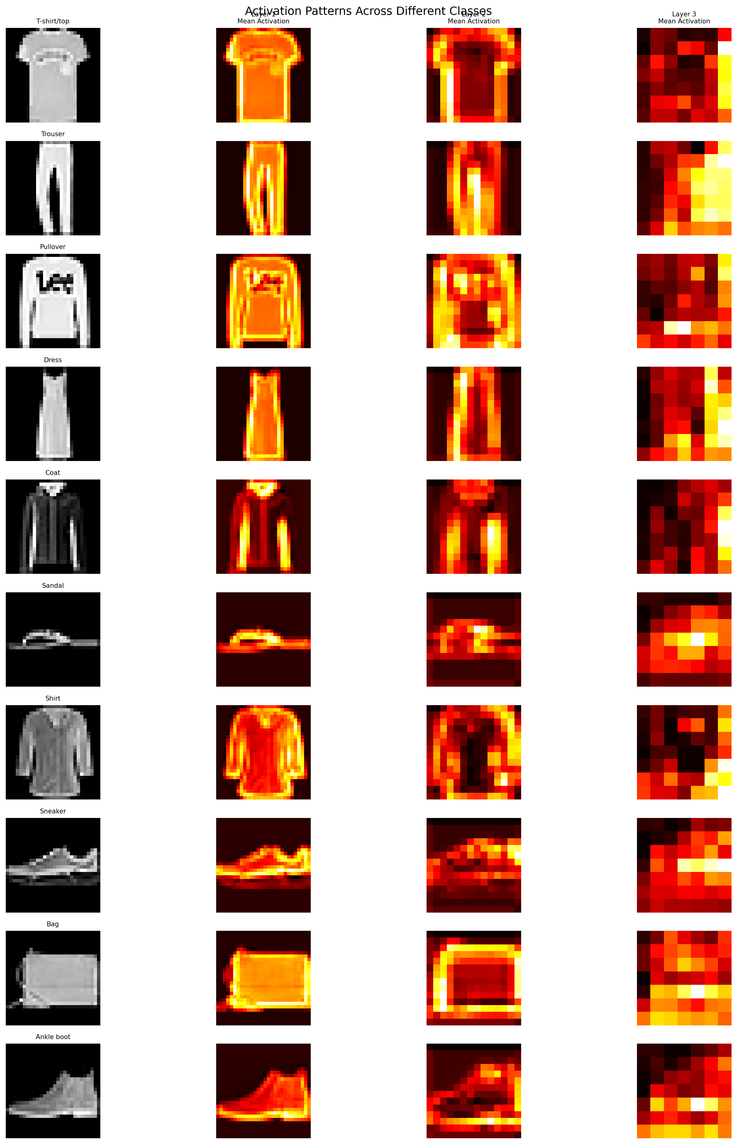
6.7 Advanced Networks for image processing
Convolutional Neural Networks (CNNs) are a class of deep learning models that have shown remarkable performance in image-related tasks. They are designed to automatically and adaptively learn spatial hierarchies of features from input images, making them particularly effective for tasks such as image classification, object detection, and image generation. A simple example of CNN for classifying MNIST Fashion dataset can be implemented as follows:
# Step 1: Import necessary librariesimport numpy as npimport matplotlib.pyplot as pltimport tensorflow as tffrom tensorflow import kerasfrom tensorflow.keras import layersfrom tensorflow.keras.models import Modelimport matplotlib.gridspec as gridspec# Step 2: Load and preprocess Fashion-MNIST datasetprint("Loading Fashion-MNIST dataset...")fashion_mnist = keras.datasets.fashion_mnist(train_images, train_labels), (test_images, test_labels) = fashion_mnist.load_data()# Class names for Fashion-MNISTclass_names = ['T-shirt/top', 'Trouser', 'Pullover', 'Dress', 'Coat','Sandal', 'Shirt', 'Sneaker', 'Bag', 'Ankle boot']# Normalize pixel values to [0, 1]train_images = train_images.astype('float32') /255.0test_images = test_images.astype('float32') /255.0# Reshape images to add channel dimension (28, 28, 1)train_images = train_images.reshape(train_images.shape[0], 28, 28, 1)test_images = test_images.reshape(test_images.shape[0], 28, 28, 1)print(f"Training data shape: {train_images.shape}")print(f"Test data shape: {test_images.shape}")# Step 3: Display sample images from the datasetdef display_sample_images(images, labels, num_rows=2, num_cols=5): plt.figure(figsize=(10, 4))for i inrange(num_rows * num_cols): plt.subplot(num_rows, num_cols, i+1) plt.imshow(images[i].reshape(28, 28), cmap='gray') plt.title(class_names[labels[i]]) plt.axis('off') plt.tight_layout() plt.suptitle('Sample Fashion-MNIST Images', y=1.02, fontsize=14) plt.show()display_sample_images(train_images, train_labels)# Step 4: Build the CNN model using Functional API instead of Sequential# This approach makes it easier to extract intermediate layer outputsdef create_cnn_functional_model():# Define input layer inputs = keras.Input(shape=(28, 28, 1), name='input')# First Convolutional Block x = layers.Conv2D(32, (3, 3), activation='relu', padding='same', name='conv1')(inputs) x = layers.MaxPooling2D((2, 2), name='pool1')(x)# Second Convolutional Block x = layers.Conv2D(64, (3, 3), activation='relu', padding='same', name='conv2')(x) x = layers.MaxPooling2D((2, 2), name='pool2')(x)# Third Convolutional Block x = layers.Conv2D(128, (3, 3), activation='relu', padding='same', name='conv3')(x) x = layers.MaxPooling2D((2, 2), name='pool3')(x)# Flatten and Dense layers x = layers.Flatten(name='flatten')(x) x = layers.Dense(128, activation='relu', name='dense1')(x) x = layers.Dropout(0.5, name='dropout')(x) outputs = layers.Dense(10, activation='softmax', name='output')(x)# Create model model = keras.Model(inputs=inputs, outputs=outputs, name='fashion_cnn')return model# Create the modelmodel = create_cnn_functional_model()model.summary()# Step 5: Compile and train the modelmodel.compile(optimizer='adam', loss='sparse_categorical_crossentropy', metrics=['accuracy'])print("\nTraining the model...")history = model.fit(train_images, train_labels, epochs=3, # Reduced epochs for faster execution batch_size=64, validation_split=0.2, verbose=0)# Step 6: Evaluate the modeltest_loss, test_accuracy = model.evaluate(test_images, test_labels, verbose=0)print(f"\nTest accuracy: {test_accuracy:.4f}")# Step 7: Create feature extraction modeldef create_feature_extractor(model):""" Create a model that extracts features from intermediate layers """# Define the layers we want to extract layer_names = ['conv1', 'conv2', 'conv3'] layer_outputs = [model.get_layer(name).output for name in layer_names]# Create feature extractor model feature_extractor = Model(inputs=model.input, outputs=layer_outputs)return feature_extractor# Create feature extractorfeature_extractor = create_feature_extractor(model)# Step 8: Visualize feature maps for a single imagedef visualize_feature_maps(image, label, feature_extractor, layer_names=['conv1', 'conv2', 'conv3']):""" Visualize feature maps from different layers """# Get feature maps feature_maps = feature_extractor.predict(image[np.newaxis, ...], verbose=0)# If only one layer output, wrap in listifnotisinstance(feature_maps, list): feature_maps = [feature_maps]# Create figure fig = plt.figure(figsize=(15, 10))# Plot original image plt.subplot(4, 4, 1) plt.imshow(image.reshape(28, 28), cmap='gray') plt.title(f'Original: {class_names[label]}', fontsize=10) plt.axis('off')# Plot feature maps for each layerfor layer_idx, (layer_name, features) inenumerate(zip(layer_names, feature_maps)):# Show 5 feature maps from this layer num_features =min(5, features.shape[-1])for i inrange(num_features): plot_idx = layer_idx *5+ i +2if plot_idx <=16: # Ensure we don't exceed subplot grid plt.subplot(4, 4, plot_idx) plt.imshow(features[0, :, :, i], cmap='viridis') plt.axis('off')if i ==0: plt.title(f'{layer_name}', fontsize=10)# Hide empty subplotsfor i inrange(len(layer_names)*5+2, 17): plt.subplot(4, 4, i) plt.axis('off') plt.suptitle('Feature Maps: From Edges to High-Level Features', fontsize=14, y=0.98) plt.tight_layout() plt.show()# Step 9: Demonstrate feature hierarchydef demonstrate_feature_hierarchy(feature_extractor, test_images, test_labels, num_samples=2):""" Demonstrate feature hierarchy for multiple sample images """print("\n"+"="*70)print("FEATURE HIERARCHY DEMONSTRATION")print("="*70)# Select random samples indices = np.random.choice(len(test_images), num_samples, replace=False)for idx in indices: image = test_images[idx] label = test_labels[idx]# Get prediction from original model prediction = model.predict(image[np.newaxis, ...], verbose=0) pred_class = np.argmax(prediction) confidence = np.max(prediction)print(f"\nImage {idx}: True class = {class_names[label]}")print(f"Predicted: {class_names[pred_class]} (confidence: {confidence:.3f})")# Visualize feature maps visualize_feature_maps(image, label, feature_extractor)# Run the demonstrationdemonstrate_feature_hierarchy(feature_extractor, test_images, test_labels, num_samples=2)# Step 10: Visualize learned filtersdef visualize_learned_filters(model, layer_name='conv1'):""" Visualize the learned filters from a convolutional layer """ layer = model.get_layer(layer_name) weights = layer.get_weights()[0] # Get the kernels# Normalize weights for better visualization weights = (weights - weights.min()) / (weights.max() - weights.min() +1e-8) num_filters =min(16, weights.shape[-1]) num_rows = (num_filters +3) //4 plt.figure(figsize=(12, 3*num_rows))for i inrange(num_filters): plt.subplot(num_rows, 4, i+1) plt.imshow(weights[:, :, 0, i], cmap='viridis') plt.axis('off') plt.title(f'Filter {i+1}', fontsize=8) plt.suptitle(f'Learned Filters from {layer_name} Layer', fontsize=14, y=0.98) plt.tight_layout() plt.show()print("\n"+"="*70)print("VISUALIZING LEARNED FILTERS")print("="*70)visualize_learned_filters(model, 'conv1')# Step 11: Show feature map statisticsdef analyze_feature_statistics(feature_extractor, sample_image, sample_label):""" Analyze and compare feature maps across layers """ layer_names = ['conv1', 'conv2', 'conv3'] feature_maps = feature_extractor.predict(sample_image[np.newaxis, ...], verbose=0)ifnotisinstance(feature_maps, list): feature_maps = [feature_maps] fig, axes = plt.subplots(1, 4, figsize=(16, 4))# Original image axes[0].imshow(sample_image.reshape(28, 28), cmap='gray') axes[0].set_title(f'Input: {class_names[sample_label]}') axes[0].axis('off')# Statistics for each layerfor i, (layer_name, features) inenumerate(zip(layer_names, feature_maps)):# Calculate mean activation across all feature maps mean_activation = np.mean(features[0], axis=-1) im = axes[i+1].imshow(mean_activation, cmap='hot') axes[i+1].set_title(f'{layer_name}\nMean Activation') axes[i+1].axis('off') plt.colorbar(im, ax=axes[i+1]) plt.suptitle('Feature Map Statistics Across Layers', fontsize=14) plt.tight_layout() plt.show()# Demonstrate with a samplesample_idx =10print(f"\nFeature statistics for {class_names[test_labels[sample_idx]]}:")analyze_feature_statistics(feature_extractor, test_images[sample_idx], test_labels[sample_idx])# Step 12: Training history visualizationdef plot_training_history(history):""" Plot training and validation accuracy/loss """ fig, (ax1, ax2) = plt.subplots(1, 2, figsize=(14, 5))# Accuracy ax1.plot(history.history['accuracy'], label='Training Accuracy', marker='o') ax1.plot(history.history['val_accuracy'], label='Validation Accuracy', marker='o') ax1.set_title('Model Accuracy') ax1.set_xlabel('Epoch') ax1.set_ylabel('Accuracy') ax1.legend() ax1.grid(True)# Loss ax2.plot(history.history['loss'], label='Training Loss', marker='o') ax2.plot(history.history['val_loss'], label='Validation Loss', marker='o') ax2.set_title('Model Loss') ax2.set_xlabel('Epoch') ax2.set_ylabel('Loss') ax2.legend() ax2.grid(True) plt.tight_layout() plt.show()plot_training_history(history)# Step 13: Comprehensive feature hierarchy explanationdef explain_feature_hierarchy_comprehensive(feature_extractor, test_images, test_labels):""" Provide a comprehensive explanation of feature hierarchy with examples """print("\n"+"="*80)print("UNDERSTANDING CNN FEATURE HIERARCHY")print("="*80) explanation =""" HOW CNNs LEARN HIERARCHICAL FEATURES: 🔵 LAYER 1 (conv1) - LOW-LEVEL FEATURES: • Detects simple patterns like edges (horizontal, vertical, diagonal) • Identifies corners and basic textures • These are universal feature detectors (similar across all images) • Feature maps show edge-like activations • Output size: 14x14 with 32 channels 🟢 LAYER 2 (conv2) - MID-LEVEL FEATURES: • Combines edges to form shapes (circles, rectangles, patterns) • Learns textures and repeating patterns • Starts recognizing object parts (sleeves, collars, straps) • Feature maps show pattern-like activations • Output size: 7x7 with 64 channels 🔴 LAYER 3 (conv3) - HIGH-LEVEL FEATURES: • Learns complex, task-specific features • Detects complete object parts and their arrangements • Features become more abstract and semantically meaningful • Feature maps show object-part activations • Output size: 3x3 with 128 channels ⚪ DENSE LAYERS - CLASSIFICATION: • Combines high-level features • Makes final classification decisions • Learns which feature combinations indicate specific clothing items """print(explanation)# Show examples of feature progressionprint("\n"+"-"*60)print("EXAMPLE: Feature progression for different clothing items")print("-"*60)# Select examples from different classes example_indices = [0, 2, 5, 9] # T-shirt, Pullover, Sandal, Ankle boot fig, axes = plt.subplots(4, 5, figsize=(20, 16))for row, idx inenumerate(example_indices): image = test_images[idx] label = test_labels[idx]# Get feature maps feature_maps = feature_extractor.predict(image[np.newaxis, ...], verbose=0)ifnotisinstance(feature_maps, list): feature_maps = [feature_maps]# Original image axes[row, 0].imshow(image.reshape(28, 28), cmap='gray') axes[row, 0].set_title(f'{class_names[label]}\nOriginal', fontsize=10) axes[row, 0].axis('off')# Feature maps from each layerfor col, (layer_name, features) inenumerate(zip(['conv1', 'conv2', 'conv3'], feature_maps)):# Show first 4 feature maps as examplesfor f inrange(min(4, features.shape[-1])): col_idx = col*4+ f +1if col_idx <5: # Ensure we don't exceed subplot grid axes[row, col_idx].imshow(features[0, :, :, f], cmap='viridis') axes[row, col_idx].set_title(f'{layer_name}\nF{f}', fontsize=8) axes[row, col_idx].axis('off') plt.suptitle('Feature Progression Across Layers for Different Clothing Items', fontsize=14, y=0.98) plt.tight_layout() plt.show()explain_feature_hierarchy_comprehensive(feature_extractor, test_images, test_labels)# Step 14: Visualize activation patternsdef visualize_activation_patterns(feature_extractor, test_images, test_labels):""" Visualize how different classes activate different feature maps """# Select one image from each class class_examples = []for class_id inrange(10): idx = np.where(test_labels == class_id)[0][0] class_examples.append((test_images[idx], class_id)) fig, axes = plt.subplots(10, 4, figsize=(16, 20))for row, (image, label) inenumerate(class_examples):# Get feature maps feature_maps = feature_extractor.predict(image[np.newaxis, ...], verbose=0)ifnotisinstance(feature_maps, list): feature_maps = [feature_maps]# Original image axes[row, 0].imshow(image.reshape(28, 28), cmap='gray') axes[row, 0].set_title(f'{class_names[label]}', fontsize=8) axes[row, 0].axis('off')# Show mean activation for each layerfor col, features inenumerate(feature_maps): mean_activation = np.mean(features[0], axis=-1) axes[row, col+1].imshow(mean_activation, cmap='hot')if row ==0: axes[row, col+1].set_title(f'Layer {col+1}\nMean Activation', fontsize=8) axes[row, col+1].axis('off') plt.suptitle('Activation Patterns Across Different Classes', fontsize=14, y=0.98) plt.tight_layout() plt.show()print("\n"+"="*70)print("CLASS-SPECIFIC ACTIVATION PATTERNS")print("="*70)visualize_activation_patterns(feature_extractor, test_images, test_labels)# Step 15: Final summaryprint("\n"+"="*70)print("SUMMARY: CNN FEATURE LEARNING HIERARCHY")print("="*70)print("""✅ Layer 1 (conv1): Edge and Corner Detectors • Responds to simple patterns • Universal feature detectors • Visualized as oriented edges✅ Layer 2 (conv2): Pattern and Shape Detectors • Combines edges into shapes • Learns textures and patterns • Starts recognizing object parts✅ Layer 3 (conv3): Object Part Detectors • Learns complex, task-specific features • Responds to semantic concepts • Abstract representations✅ Dense Layers: Classifiers • Combines high-level features • Makes final classification decisions • Learns class-specific feature combinationsThe network progressively builds more abstract and task-specific representations from raw pixels to final classification decisions.""")# Save the modelmodel.save('fashion_mnist_functional_model.h5')print("\nModel saved as 'fashion_mnist_functional_model.h5'")
Loading Fashion-MNIST dataset...
Training data shape: (60000, 28, 28, 1)
Test data shape: (10000, 28, 28, 1)
WARNING:absl:You are saving your model as an HDF5 file via `model.save()` or `keras.saving.save_model(model)`. This file format is considered legacy. We recommend using instead the native Keras format, e.g. `model.save('my_model.keras')` or `keras.saving.save_model(model, 'my_model.keras')`.
======================================================================
SUMMARY: CNN FEATURE LEARNING HIERARCHY
======================================================================

✅ Layer 1 (conv1): Edge and Corner Detectors
   • Responds to simple patterns
   • Universal feature detectors
   • Visualized as oriented edges

✅ Layer 2 (conv2): Pattern and Shape Detectors
   • Combines edges into shapes
   • Learns textures and patterns
   • Starts recognizing object parts

✅ Layer 3 (conv3): Object Part Detectors
   • Learns complex, task-specific features
   • Responds to semantic concepts
   • Abstract representations

✅ Dense Layers: Classifiers
   • Combines high-level features
   • Makes final classification decisions
   • Learns class-specific feature combinations

The network progressively builds more abstract and
task-specific representations from raw pixels to
final classification decisions.


Model saved as 'fashion_mnist_functional_model.h5'
This capstone project synthesizes concepts from all five modules:
Module 1: Linear constraints and formulations
Module 2: Nonlinear cost modeling
Module 3: Project planning and scheduling
Module 4: Graph algorithms and network optimization
Module 5: Machine learning and gradient optimization
6.8.1.2 Project Vision
Develop an intelligent campus optimization system that:
Predicts facility demands using machine learning
Optimizes resource allocation using advanced algorithms
Adapts to changing conditions in real-time
Visualizes optimal solutions and provides insights
6.8.1.3 System Architecture
Data Layer:
Historical campus operations data
Real-time sensor data
Environmental and contextual data
Model Layer:
Demand prediction models
Optimization algorithms
Constraint handlers
Application Layer:
Dashboard for campus operations
Real-time optimization engine
Reporting and analytics
6.8.2 Capstone Project Requirements
6.8.2.1 Part A: Predictive Modeling (5 Marks)
Objective: Develop machine learning models to predict campus facility demands.
Tasks:
Feature Engineering:
Temporal features (hour, day, month, holidays)
Environmental features (weather, temperature)
Event features (exams, sports, cultural events)
Historical demand patterns
Model Development:
Time series forecasting models
Regression models for demand prediction
Ensemble methods for improved accuracy
Optimization Integration:
Use predictions as input to optimization models
Handle prediction uncertainty in optimization
Adaptive models that update with new data
6.8.2.2 Part B: Integrated Optimization System (6 Marks)
Objective: Create a comprehensive optimization system that uses predictions to make optimal decisions.
Tasks:
Multi-Period Optimization:
Dynamic optimization across time horizons
Handling of time-dependent constraints
Integration of predicted vs actual demands
Stochastic Optimization:
Handle uncertainty in predictions
Robust optimization approaches
Scenario-based planning
Real-Time Adaptation:
Update optimization based on real-time data
Handle unexpected events and disruptions
Provide alternative solutions
6.8.2.3 Part C: Advanced Algorithm Implementation (5 Marks)
Objective: Implement sophisticated optimization algorithms for complex campus problems.
Tasks:
Gradient-Based Optimization:
Implement Adam optimizer for parameter tuning
Learning rate scheduling and adaptation
Handling of non-convex objective functions
Metaheuristic Integration:
Combine gradient methods with heuristic approaches
Hybrid algorithms for complex constraints
Multi-objective optimization techniques
Large-Scale Optimization:
Distributed optimization approaches
Parallel processing for campus-scale problems
Efficient data structures for optimization
6.8.2.4 Part D: System Deployment & Evaluation (4 Marks)
Objective: Deploy and evaluate the complete system.
Tasks:
Performance Metrics:
Optimization solution quality
Computational efficiency
Prediction accuracy
Practical feasibility
Comparative Analysis:
Baseline vs optimized solutions
Different algorithm comparisons
Sensitivity to parameter choices
Business Impact Assessment:
Cost savings quantification
Service improvement metrics
Environmental impact reduction
Scalability assessment
6.8.3 Sample Capstone Problem
Problem Statement: Develop an AI-driven system for Campus City that:
Predicts hourly demands for all 15 facilities
Optimizes warehouse operations and delivery schedules
Adapts to real-time events (emergencies, weather)
Provides dashboard for operations management
Solution Components:
Prediction Module:
LSTM neural networks for time series prediction
Gradient-based optimization for model training
Uncertainty quantification for predictions
Optimization Module:
Multi-period mixed-integer programming
Stochastic optimization for demand uncertainty
Real-time re-optimization engine
Integration Layer:
API for data exchange between modules
Visualization dashboard
Alert system for exceptional situations
6.8.4 Capstone Design Questions
How would you design a neural network architecture for predicting campus facility demands that captures both temporal patterns and external factors?
What gradient optimization method would you choose for training your prediction models and why?
How would you handle the trade-off between prediction model complexity and optimization solution time in a real-time system?
Design a multi-objective optimization approach that balances cost minimization with service level maximization for campus operations.
How would you validate that your AI-enhanced optimization system actually improves campus operations compared to traditional methods?
6.9 Review Questions
Describe the concept of regularization in the machine learning context. Given any three commonly used regularization in regression models.
Explain the concept of momentum in loss optimization, providing a clear rationale. Also, write the algorithm for the momentum method.
Explain the bias-variance trade-off in machine learning. How does it relate to model complexity and generalization?
What is the purpose of a validation set in machine learning, and how does it differ from the training and test sets?
Describe the concept of overfitting in machine learning. What are some common techniques to prevent overfitting?
Explain the concept of cross-validation and how it can be used to evaluate the performance of a machine learning model.
Explain the gradient descent method for minimizing the loss function. What are the common issues with this method, and suggest a method to overcome them?
Minimize the quadratic function \(f(x)= x^2- 4x + 4\) using gradient descent with momentum starting from \(x_0= 0\), with learning rate \(\eta = 0.1\) and \(\gamma=0.9\) in 4 iterations.
What is the effect of the learning rate on gradient descent convergence? Provide examples of problems caused by too large and too small learning rates.
Compare RMSProp and Adam optimizers. When would you choose one over the other for campus demand prediction?
Explain how momentum helps gradient descent overcome oscillations in narrow valleys.
Minimize the quadratic function \(f(x)= x^2- 4x + 4\) using gradient descent starting from \(x_0= 0\), with learning rate \(\eta = 0.1\) in 4 iterations.
Explain different types of gradient descent methods and compare them with any three dominant advantages and disadvantages.
Let \(y_i\) be the ground truth and \(\hat{y}_i\) be the predicted value of a functional approximation \(y = f(\theta_0 + \theta_1 x)\), where \(\theta_0, \theta_1\) are parameters. Formulate the mean square error for this predictive function, considering \(n\) samples. Also derive the update formula for both \(\theta_0\) and \(\theta_1\) using the gradient descent method.
Explain the concept of learning rate in gradient descent. What are the potential consequences of choosing a learning rate that is too high or too low?
Describe the Adam optimization algorithm and explain how it combines the advantages of both momentum and RMSProp.
Explain the concept of stochastic optimization and how it differs from traditional optimization methods. Provide an example of a stochastic optimization algorithm.
Discuss the challenges of integrating AI techniques with traditional optimization methods. How can these challenges be addressed in practice?
6.10 Module 5 Summary
6.10.1 Key Concepts Mastered
✅ Gradient descent fundamentals and mathematical foundations
System Integration: Combining prediction models with optimization
Practical Implementation: Applying advanced methods to campus-scale problems
6.10.3 Course Integration
This module completes the learning journey by:
Building on foundations from previous modules
Introducing cutting-edge optimization techniques
Preparing students for real-world AI/ML optimization challenges
Providing a comprehensive skill set for industry applications
6.10.4 Career Applications
Skills developed in this module are directly applicable to:
Data Scientist roles in logistics and operations
Machine Learning Engineer positions
Optimization Specialist careers
AI Product Development
Research in computational optimization
6.10.5 Final Preparation
Complete Capstone Project integration
Review all module concepts for final assessment
Prepare professional portfolio with project work
Develop presentation skills for technical solutions
6.11 Course Culmination
6.11.1 Learning Journey Recap
Module 1: Mathematical foundations and linear optimization
Module 2: Nonlinear methods and constraint handling
Module 3: Project planning and heuristic approaches
Module 4: Combinatorial optimization and graph algorithms
Module 5: AI integration and advanced optimization
6.11.2 Professional Competencies Achieved
Technical Expertise: From basic LP to neural network optimization
Problem-Solving: Structured approach to complex optimization challenges
Implementation Skills: Python proficiency with industry-standard libraries
Business Acumen: Translating technical solutions to business value
Communication: Presenting optimization insights to diverse audiences
6.11.3 Future Learning Pathways
Advanced topics in convex optimization
Reinforcement learning for sequential decision making
Quantum optimization algorithms
Large-scale distributed optimization systems
Research in optimization theory and applications
This module completes the Computational Optimization & Applications course, equipping students with comprehensive optimization skills applicable to the most challenging problems in technology, business, and research.