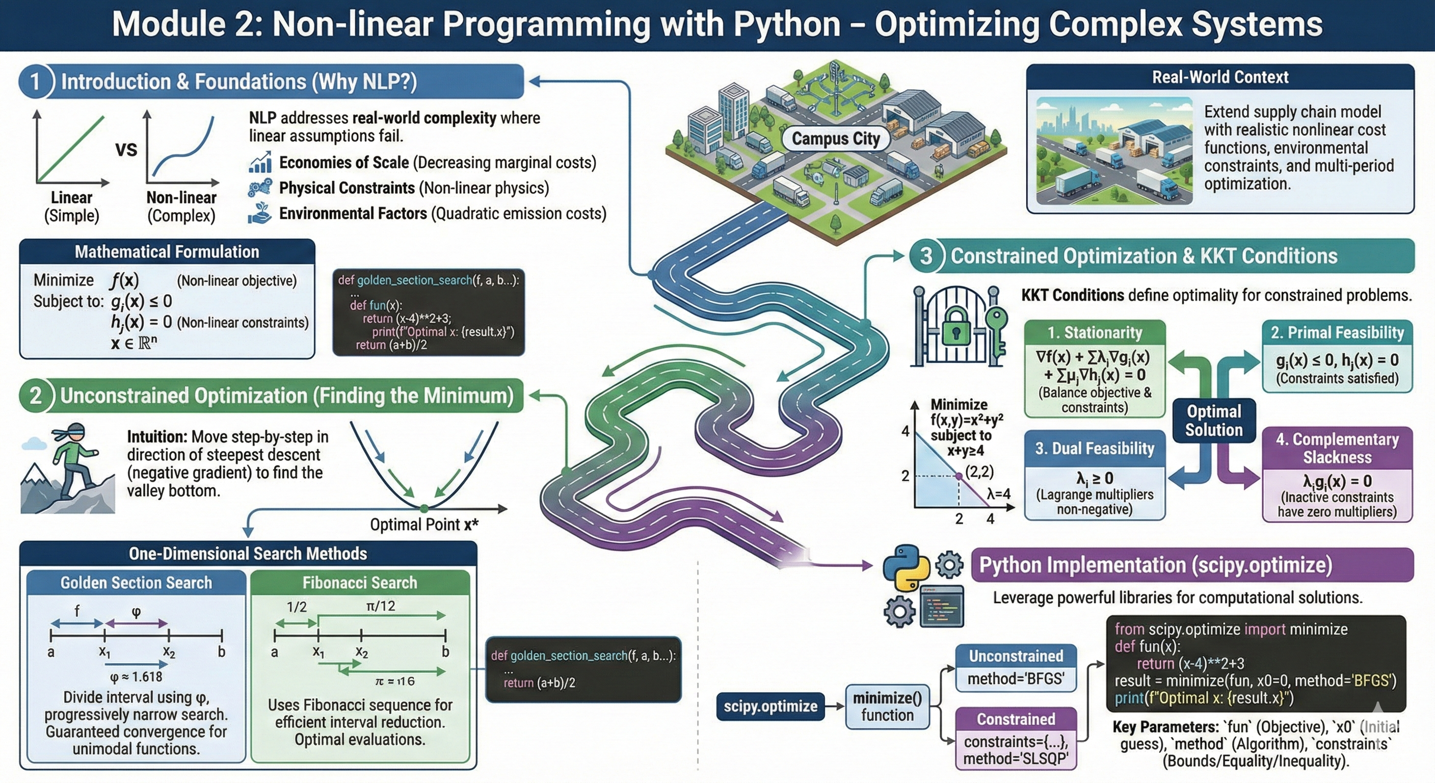
Extend the Campus City supply chain model with realistic nonlinear cost functions, environmental constraints, and multi-period optimization challenges.
3.2 Introduction to Nonlinear Optimization
Nonlinear programming (NLP) is an optimization technique used to find the best outcome (maximum profit, lowest cost, etc.) in a mathematical model where at least one of the objective functions or constraints is nonlinear . This means the relationship between variables cannot be represented on a straight line. NLP addresses the complexity found in real-world scenarios, such as modeling physical systems or financial markets, where linear assumptions are often inadequate for accurate prediction and decision-making . Key components of an NLP problem include decision variables, an objective function to be optimized, and constraints that limit the possible solutions.
The primary purpose of using NLP is to provide more accurate and realistic models for optimization problems across various fields, including engineering design, economics, finance, and operations research. For example, in portfolio optimization, investors use NLP to maximize returns while balancing risk, which inherently involves nonlinear relationships between different assets. In chemical engineering, NLP helps optimize process yields and efficiency where reaction kinetics are nonlinear. It is applied when linear models fail to capture the true nature of the relationships between the inputs and outputs of a system.
Solving NLP problems involves specialized algorithms, such as sequential quadratic programming (SQP), interior-point methods, or generalized reduced gradient methods. The “how much” refers to the computational resources and mathematical complexity required, which are often significantly greater than for linear programming. The complexity and effort vary widely based on the problem’s size and structure (e.g., convexity). While the general approach is similar (define variables, objective, constraints), the execution demands sophisticated software and potentially substantial processing power to find the global optimum efficiently.
3.2.1 Theoretical Foundation
The fundamental theoretical difference between Linear Programming Problems (LPP) and NLP lies in the mathematical nature of their objective functions and constraints, which dictates the complexity of their feasible regions, solution methods, and optimality guarantees.
Feature
Linear Programming (LPP)
Nonlinear Programming (NLP)
Function Types
Objective function and all constraints must be linear.
At least one function (objective or a constraint) is nonlinear.
Feasible Region
The feasible region is a convex polyhedron (a shape with flat faces).
The feasible region can be non-convex, curved, or disconnected.
Optimality
A locally optimal solution is always a globally optimal solution. The optimum lies at a corner point (vertex) of the feasible region.
Solutions often only guarantee a local optimum. The global optimum is difficult to find without additional assumptions (e.g., convexity of the entire problem).
Solution Methods
Solved primarily by the Simplex Method or Interior Point Methods, which systematically explore the corner points.
Requires more complex iterative numerical methods such as Gradient Descent, Newton’s Method, or Lagrangian heuristics, often relying on derivatives.
Computational Complexity
Generally easier and faster to solve, even with a vast number of variables.
Generally more computationally intensive and difficult to solve, especially for large-scale, non-convex problems.
                     ┌───────────────────────────────────────────┐
                     |      Optimization Problems                |
                     └───────────────────────────────────────────┘
                                    |
                ┌───────────────────┴───────────────────┐
                |                                       |
     ┌───────────────────────┐               ┌────────────────────────┐
     | Linear Programming     |               | Nonlinear Programming  |
     | (LPP)                  |               | (NLP)                  |
     └───────────────────────┘               └────────────────────────┘
                |                                       |
     ┌───────────────────────┐               ┌────────────────────────────────┐
     | Linear objective &     |               | At least one objective or      |
     | linear constraints     |               | constraint is nonlinear        |
     └───────────────────────┘               └────────────────────────────────┘
                |                                       |
      Feasible region is convex                Region may be curved or nonconvex
                |                                       |
    Optimal solution at a vertex                May have multiple local optima
                |                                       |
    Solved via Simplex / IPM                      Solved via numerical methods
3.2.1.1 Why Nonlinear Optimization?
Linear programming assumes proportional relationships, but real-world problems often involve:
Economies of scale: Decreasing marginal costs
Physical constraints: Nonlinear relationships (distance vs fuel consumption)
Quality constraints: Minimum/maximum thresholds with nonlinear effects
Environmental factors: Quadratic cost functions for emissions
Problem Statement: A delivery company has a cost function \(C(d) = 500 + 2d + 0.1d^2\) where \(d\) is distance in km. Find the optimal delivery distance that minimizes cost per unit for a shipment of 100 units.
Check boundaries: Minimum at \(d = 0\) with cost $5/unit
Interpretation: The cost function is convex and increasing, so minimum occurs at shortest distance.
3.2.3 Review Questions
What are three real-world scenarios where linear models fail and nonlinear optimization is required?
Explain the difference between convex and non-convex optimization problems. Why is this distinction important?
A manufacturing process has cost \(C(x) = 1000 + 50x + 0.5x^2\) where x is production volume. Find the production level that minimizes average cost.
Why can’t the Simplex method be directly applied to nonlinear optimization problems?
Describe a campus logistics scenario where nonlinear optimization would provide better results than linear programming.
NLP Vs LPP
The linear nature of LPP guarantees a single, well-defined feasible region and objective function behavior, allowing for robust algorithms like the Simplex method to efficiently find the absolute best (global) solution. NLP, by contrast, accommodates the complex, often non-convex, relationships found in many real-world problems. This flexibility comes at a theoretical and computational cost: the presence of curves and non-linear interactions means there may be multiple “local” optimal points, and standard algorithms may get stuck at one that is not the overall best solution. The theoretical foundation of NLP thus focuses heavily on iterative improvement, convergence properties, and finding efficient ways to navigate these more challenging landscapes.
3.3 Unconstrained Optimization Methods
Unconstrained Nonlinear Programming deals with optimizing a nonlinear objective function without any constraints on the decision variables. The objective is to determine a point \(x^{*} \in \mathbb{R}^{n}\) such that:
\[
\min_{x \in \mathbb{R}^{n}} f(x)
\]
(or equivalently \(\max f(x)\) depending on the problem context).
Intuition Behind Unconstrained NLP
The central idea in solving unconstrained NLP problems is to understand how the objective function surface behaves and to iteratively move toward regions where the function value improves.
Downhill Movement Intuition
For minimization problems, the objective is to move step-by-step in a direction that decreases the function value, much like descending a slope.
Hiking Analogy
Consider attempting to reach the lowest valley point in a mountainous landscape while blindfolded. The only available information is the slope beneath your feet. The safest strategy is always stepping in the direction that slopes downward most strongly.
Key points
This direction of steepest descent is mathematically represented by the gradient \(\nabla f(x)\).
Repeated movement in this direction leads to progressively lower function values until a flat region is encountered. ## Link with Calculus
In single-variable calculus, stationary (optimal) points are found by solving:
\[
\frac{df}{dx} = 0
\]
In multi-variable calculus, this concept generalizes to:
\[
\nabla f(x^{*}) = 0
\]
A point where the gradient is zero is called a critical point. It may represent:
Type of Critical Point
Interpretation
Local Minimum
Valley bottom
Local Maximum
Hilltop
Saddle Point
A flat ridge point
To classify these points, second-order information is required.
First-Order Necessary Condition (FONC)
For a differentiable function \(f(x)\), a point \(x^{*}\) can be a local minimum only if:
\[
\nabla f(x^{*}) = 0
\]
This guarantees flatness but does not guarantee an actual minimum.
Second-Order Sufficient Condition (SOSC)
Let \(H(x)\) denote the Hessian matrix of second partial derivatives:
If \(x^{*}\) satisfies \(\nabla f(x^{*}) = 0\) and
\[
H(x^{*}) \text{ is positive definite}
\]
then \(x^{*}\) is a strict local minimum.
Curvature Interpretation
Hessian Property
Interpretation
\(H \succ 0\)
Strict minimum (upward curvature)
\(H \prec 0\)
Maximum (downward curvature)
Indefinite
Saddle point (mixed curvature)
3.3.1 Algorithms for Unconstrained NLP
This module focuses specifically on iteration-based direct search techniques, which do not require gradient or Hessian calculations. Such algorithms are especially useful when:
The derivative is difficult or impossible to compute
The objective function is noisy or discontinuous
Only function value evaluations are available
The algorithms covered in this module include:
3.3.1.1 Fibonacci Search Method
A bracketing method used for one-dimensional minimization.
This method iteratively narrows down an interval containing the minimum using Fibonacci numbers.
Key Concept
The interval size decreases proportionally according to Fibonacci sequence ratios, ensuring efficient narrowing.
This method is applicable to Smooth 1-D unimodal functions.
3.3.1.2 Golden Section Search Method
A more efficient improvement over Fibonacci search, eliminating the need to precompute steps.
The method divides the interval using the Golden Ratio:
\[
\phi = \frac{\sqrt{5} + 1}{2} \approx 1.618
\]
Key Concept
The interval is repeatedly reduced while maintaining internal division based on \(\phi\), ensuring optimal reduction at each iteration.
3.3.1.3 Hooke and Jeeves Pattern Search Method
A direct search method used for multidimensional optimization without derivatives.
Key Components
Exploratory search: Tests moves along coordinate directions to find improvement.
Pattern move: Accelerates search in the identified promising direction.
3.3.1.4 Advantages
Does not require derivative information
Suitable for complex, non-smooth landscapes
Unconstrained NLP is guided by theoretical optimality conditions and solved computationally using iterative search techniques. In this module, emphasis is placed on direct search algorithms useful when derivatives are unavailable.
The practical tools studied—Fibonacci Search, Golden Section Search, and Hooke & Jeeves—offer systematic methods for approaching optimal points when classical derivative-based methods cannot be applied.
3.3.1.5 Review Questions
Why does the condition \(\nabla f(x^{*}) = 0\) not guarantee a minimum?
What role does curvature play in distinguishing minima from maxima?
Why are direct search methods such as Fibonacci or Golden Section useful?
Compare Hooke & Jeeves with gradient-based methods.
Explain why Golden Section is more efficient than Fibonacci Search.
3.3.2 Theoretical Foundation
3.3.2.1 One-Dimensional Search Methods
When dealing with single-variable nonlinear functions, we use specialized search techniques:
Golden Section Search: - Divide interval using golden ratio \(\phi = \frac{1+\sqrt{5}}{2} \approx 1.618\) - Progressively narrow search interval - Guaranteed convergence for unimodal functions
Fibonacci Search: - Uses Fibonacci sequence for interval reduction - Optimal in terms of function evaluations - Similar convergence properties to Golden Section
3.3.2.2 Mathematical Basis
For a unimodal function \(f(x)\) on interval ([a,b]):
Golden Section Points:\[
\begin{aligned}
x_1 & = b - \frac{b-a}{\phi} \\
x_2 & = a + \frac{b-a}{\phi}
\end{aligned}
\]
Where \(\phi=1.618\)
Alter:
Instead of choosing \(\phi=1.618\), we can select the other Golder section ratio (\(<1\)). In that case the section points can be calculated as: \[
\begin{aligned}
x_1 & = b - \phi\cdot (b-a) \\
x_2 & = a + \phi\cdot (b-a)
\end{aligned}
\]
Iteration: Compare \(f(x_1)\) and \(f(x_2)\), eliminate portion of interval based on which is larger.
3.3.3 Sample Problem 1
Problem Statement: Use Golden Section search to minimize \(f(x) = (x-3)^2 + 2\) on interval [0, 5] with 4 iterations.
Since \(f(x_1) < f(x_2)\), new interval: [1.91, 3.82]
Continue for 4 iterations → Final interval: [2.85, 3.15] containing true minimum at x=3
3.3.4 Sample Problem 2
Problem Statement: A warehouse has energy consumption \(E(w) = 1000 + 50w + 0.2w^2\) kWh, where w is weekly shipments (0 ≤ w ≤ 200). Find optimal shipment volume that minimizes energy per shipment.
Solution: Energy per shipment: \(f(w) = \frac{1000}{w} + 50 + 0.2w\)
Using Golden Section on [10, 200]:
Iteration 1: Compare w=70.8 and w=139.2
Iteration 2: Compare w=44.4 and w=70.8
Iteration 3: Compare w=57.6 and w=70.8
Optimal: w ≈ 70.7 shipments/week, energy/shipment ≈ 78.3 kWh
3.3.5 Sample problem 3
Minimize \[f(x)=-\frac{1}{(x-1)^2}\left(\ln(x)-2\left(\frac{x-1}{x+1}\right)\right)\] such that \(x\) in \([1.5,4.5]\) using the Golden Section Method.
3.3.6 Review Questions
Explain why Golden Section search is more efficient than exhaustive search for unimodal functions.
Compare Golden Section and Fibonacci search methods. When would you choose one over the other?
A transportation cost function is \(C(d) = \frac{1000}{d} + 2d\) for d > 0. Use Golden Section to find the optimal distance in [10, 100] with 3 iterations.
What is a unimodal function and why is this property important for one-dimensional search methods?
How would you modify Golden Section search if you suspected multiple local minima in your search interval?
3.4 Constrained Optimization & KKT Conditions
3.4.1 Theoretical Foundation
3.4.1.1 Karush-Kuhn-Tucker (KKT) Conditions
For constrained nonlinear optimization, KKT conditions provide necessary conditions for optimality:
Primal Problem:\[
\begin{aligned}
\text{Minimize } & f(\mathbf{x}) \\
\text{Subject to } & g_i(\mathbf{x}) \leq 0, \quad i = 1, \ldots, m \\
& h_j(\mathbf{x}) = 0, \quad j = 1, \ldots, p
\end{aligned}
\]
Case 2: 4 - x - y = 0 → from stationarity: x=y=λ/2 → 4 - λ/2 - λ/2 = 0 → λ=4
Solution: x=2, y=2, λ=4, f=8
3.4.3 Sample Problem
Problem Statement: Campus City wants to minimize transportation cost \(C(d) = 2d + 0.1d^2\) while ensuring at least 80% of routes are under 3km. Formulate as KKT problem.
minimize() function: Unified interface for multiple algorithms
Algorithm choices: SLSQP, trust-constr, COBYLA for constrained problems
3.5.1.2 Key Functions
from scipy.optimize import minimize# For unconstrained problemsresult = minimize(fun, x0, method='BFGS')# For constrained problems result = minimize(fun, x0, constraints=constraints, method='SLSQP')
Practical Considerations
Initial guess (\(x_0\)): Critical for convergence
Gradient provision: Can significantly improve performance
Constraint formulation: Proper bounds and constraint objects
3.5.2 Sample Problem
Problem Statement: Implement Golden Section search in Python for \(f(x)=(x−4)^2+3\) on [0, 10].
Solution:
import mathdef golden_section_search(f, a, b, tol=1e-6, max_iter=100): phi = (1+ math.sqrt(5)) /2for i inrange(max_iter): x1 = b - (b - a) / phi x2 = a + (b - a) / phiif f(x1) > f(x2): a = x1else: b = x2ifabs(b - a) < tol:return (a + b) /2return (a + b) /2# Test the functiondef objective(x):return (x -4)**2+3result = golden_section_search(objective, 0, 10)print(f"Optimal x: {result:.4f}") # Output: Optimal x: 4.0000
Optimal x: 4.0000
3.5.3 Solution of constrained NLPP
To solve NLPP using KKT method, we will use solve() function from the sympy library. Key functions required for solution will be imported
from sympy import symbols, diff, solve
Example 1: Minimize \(f(x, y) = x^2 + y^2\) subject to \(x + y \ge 4\) (Standard form: \(4 - x - y \le 0\)).
SymPy does not inherently “solve” inequality constraints in the same way a numerical solver (like SciPy) does. Instead, you must manually transform the inequality into an equation using the Complementary Slackness condition from the KKT framework.Here is the logic: An inequality constraint \(g(x) \le 0\) is handled by introducing a Lagrange multiplier \(\lambda\) and adding the equation \(\lambda \cdot g(x) = 0\) to your system.
The 3-Step “Filter” WorkflowSince SymPy’s solve function returns all mathematical solutions (stationary points), you must add a “Filter” step to check the inequalities manually. - Formulate: Convert inequalities to KKT equations (Stationarity + Complementary Slackness). - Solve: Use solve() to find all candidate points. - Filter: Discard solutions that violate Primal Feasibility (\(g(x) \le 0\)) or Dual Feasibility (\(\lambda \ge 0\)).
Python code:
from sympy import symbols, diff, solve# 1. Define Variablesx, y = symbols('x y', real=True)lam = symbols('lambda', real=True) # Lagrange Multiplier# 2. Define Functionsf = x**2+ y**2# Objectiveg =4- x - y # Inequality constraint (g <= 0)# 3. Formulate Lagrangian# L = f + lambda * gL = f + lam * g# 4. Generate KKT Equations# A. Stationarity: Gradient of L must be zeroeq1 = diff(L, x)eq2 = diff(L, y)# B. Complementary Slackness: lambda * constraint = 0eq3 = lam * g# 5. Solve the System of Equations# We ask SymPy to find values for x, y, and lambda that satisfy these 3 equalitiessolutions = solve([eq1, eq2, eq3], (x, y, lam), dict=True)print(f"Candidate Solutions found: {len(solutions)}")# 6. Filter Solutions (The Crucial Step for Inequalities)print("\n--- Validation Step ---")valid_solutions = []for sol in solutions: x_val = sol[x] y_val = sol[y] lam_val = sol[lam]# Check Primal Feasibility: g(x) <= 0# (Using a small tolerance for floating point comparisons if needed) primal_check = (4- x_val - y_val) <=0# Check Dual Feasibility: lambda >= 0 dual_check = lam_val >=0print(f"Testing Point ({x_val}, {y_val}) with lambda={lam_val}:")print(f" Constraint g <= 0? {primal_check}")print(f" Dual lambda >= 0? {dual_check}")if primal_check and dual_check:print(" VALID Optimal Solution") valid_solutions.append(sol)else:print(" INVALID (Violates KKT conditions)")# Output Final Resultif valid_solutions: opt = valid_solutions[0]print(f"\nOptimal Solution: x={opt[x]}, y={opt[y]}, cost={opt[x]**2+ opt[y]**2}")
Candidate Solutions found: 2

--- Validation Step ---
Testing Point (0, 0) with lambda=0:
  Constraint g <= 0? False
  Dual lambda >= 0? True
 INVALID (Violates KKT conditions)
Testing Point (2, 2) with lambda=4:
  Constraint g <= 0? True
  Dual lambda >= 0? True
 VALID Optimal Solution

Optimal Solution: x=2, y=2, cost=8
Example 2: Solve \(f(x_1,x_2)=-x_1^2-x_2^2\); \(-x_1-x_2\le -1\); \(-2x_1+2x_2\le 1\); \(x_1,x_2\ge 0\).
import sympy as sp# 1. Define Variablesx1, x2 = sp.symbols('x1 x2', real=True)lam1, lam2 = sp.symbols('lambda1 lambda2', real=True)# 2. Define Objective (Maximization)f =-x1**2- x2**2# 3. Define Constraints in Standard Form (g(x) <= 0)# Original: -x1 - x2 >= -1 -> x1 + x2 <= 1 -> x1 + x2 - 1 <= 0g1 = x1 + x2 -1# Original: -2x1 + 2x2 <= 1 -> -2x1 + 2x2 - 1 <= 0g2 =-2*x1 +2*x2 -1# 4. Formulate Lagrangian for Maximization (L = f - lambda*g)L = f - lam1 * g1 - lam2 * g2# 5. KKT Equations# A. Stationarity (Gradient of L w.r.t x must be 0)stat_x1 = sp.diff(L, x1)stat_x2 = sp.diff(L, x2)# B. Complementary Slackness (lambda * g = 0)slack_1 = lam1 * g1slack_2 = lam2 * g2# 6. Solve the Systemprint("Solving KKT system...")# We assume non-negativity of x (x >= 0) is a boundary check rather than an explicit Lagrangian term # to keep the symbolic solver efficient for this demo.solutions = sp.solve([stat_x1, stat_x2, slack_1, slack_2], (x1, x2, lam1, lam2), dict=True)# 7. Validation & Filteringprint(f"\nFound {len(solutions)} candidate points. Filtering for optimality...")print("-"*75)print(f"{'Point (x1, x2)':<20} | {'Multipliers':<20} | {'Objective':<10} | {'Status'}")print("-"*75)best_f =-float('inf')best_sol =Nonefor sol in solutions:# Extract numerical values x1_v =float(sol[x1]) x2_v =float(sol[x2]) l1_v =float(sol[lam1]) l2_v =float(sol[lam2]) status ="Valid"# Check 1: Non-negativity of variables (x >= 0)if x1_v <-1e-7or x2_v <-1e-7: status ="Invalid (x < 0)"# Check 2: Primal Feasibility (g <= 0)elif (x1_v + x2_v -1) >1e-7: status ="Invalid (g1 > 0)"elif (-2*x1_v +2*x2_v -1) >1e-7: status ="Invalid (g2 > 0)"# Check 3: Dual Feasibility (lambda >= 0 for Max problem with L = f - lg)elif l1_v <-1e-7or l2_v <-1e-7: status ="Invalid (lambda < 0)"# Calculate Objective obj_val =-x1_v**2- x2_v**2print(f"({x1_v:.4f}, {x2_v:.4f}) | L1={l1_v:.4f}, L2={l2_v:.4f} | {obj_val:.4f} | {status}")if"Valid"in status and obj_val > best_f: best_f = obj_val best_sol = (x1_v, x2_v)print("-"*75)if best_sol:print(f"\n Optimal Solution: x1 = {best_sol[0]}, x2 = {best_sol[1]}")print(f" Max Objective Value = {best_f}")
Example 3: Minimize \(f(x_1,x_2)=2x_1+6x_2\) subject to \(x_1-x_2\le 0\); \(x_1^2+x_2^2\ge 4\); \(x_1,x_2\ge 0\).
Mathematical Formulation for Sympy requires constraints to be in the form \(g(x) \ge 0\). We must rearrange the given inequalities: - Objective: Minimize \(f(x) = 2x_1 + 6x_2\) - Constraint 1:\(x_1 - x_2 \le 0 \implies x_2 - x_1 \ge 0\) - Constraint 2:\(x_1^2 + x_2^2 \ge 4 \implies x_1^2 + x_2^2 - 4 \ge 0\) - Bounds:\(x_1, x_2 \ge 0\)
import sympy as sp# 1. Define Symbolsx1, x2 = sp.symbols('x1 x2', real=True)lam1, lam2 = sp.symbols('lambda1 lambda2', real=True)# 2. Define Objective (Minimization)f =2*x1 +6*x2# 3. Define Constraints in Standard Form (g(x) <= 0)# Constraint 1: x1 - x2 <= 0g1 = x1 - x2# Constraint 2: x1^2 + x2^2 >= 4 --> 4 - x1^2 - x2^2 <= 0g2 =4- x1**2- x2**2# 4. Formulate Lagrangian (Minimization: L = f + sum(lambda * g))L = f + lam1 * g1 + lam2 * g2# 5. KKT Equations# A. Stationarity (Gradient of L = 0)eq_x1 = sp.diff(L, x1)eq_x2 = sp.diff(L, x2)# B. Complementary Slackness (lambda * g = 0)eq_slack1 = lam1 * g1eq_slack2 = lam2 * g2# 6. Solve the Systemprint("Solving KKT system equations...")# This solves for stationary points and intersection pointssolutions = sp.solve([eq_x1, eq_x2, eq_slack1, eq_slack2], (x1, x2, lam1, lam2), dict=True)# 7. Filter & Validate Solutionsprint(f"\nFound {len(solutions)} candidate points. Validating KKT conditions...")print("-"*85)print(f"{'Point (x1, x2)':<20} | {'Multipliers':<20} | {'Cost':<10} | {'Status'}")print("-"*85)optimal_val =float('inf')optimal_sol =Nonefor sol in solutions:# Extract values (convert to float for comparison) x1_v =float(sol[x1]) x2_v =float(sol[x2]) l1_v =float(sol[lam1]) l2_v =float(sol[lam2])# Validation Logic status ="Valid"# 1. Domain Check (x >= 0)if x1_v <-1e-7or x2_v <-1e-7: status ="Invalid (x < 0)"# 2. Primal Feasibility (g <= 0)# Check g1: x1 - x2 <= 0elif (x1_v - x2_v) >1e-7: status ="Invalid (g1 > 0)"# Check g2: 4 - x1^2 - x2^2 <= 0elif (4- x1_v**2- x2_v**2) >1e-7: status ="Invalid (g2 > 0)"# 3. Dual Feasibility (lambda >= 0 for Minimization)elif l1_v <-1e-7or l2_v <-1e-7: status ="Invalid (lambda < 0)"# Calculate Cost cost =2*x1_v +6*x2_vprint(f"({x1_v:.4f}, {x2_v:.4f}) | L1={l1_v:.4f}, L2={l2_v:.4f} | {cost:.4f} | {status}")if"Valid"in status and cost < optimal_val: optimal_val = cost optimal_sol = (x1_v, x2_v)print("-"*85)if optimal_sol:print(f"\n Optimal Solution: x1 = {optimal_sol[0]:.4f}, x2 = {optimal_sol[1]:.4f}")print(f" Minimum Value = {optimal_val:.4f}")# Insight for the userprint("\nInsight: The solution lies at the intersection of the line x1=x2 and the circle.")
Solving KKT system equations...

Found 4 candidate points. Validating KKT conditions...
-------------------------------------------------------------------------------------
Point (x1, x2)       | Multipliers          | Cost       | Status
-------------------------------------------------------------------------------------
(-0.6325, -1.8974)   | L1=0.0000, L2=-1.5811 | -12.6491    | Invalid (x < 0)
(0.6325, 1.8974)   | L1=0.0000, L2=1.5811 | 12.6491    | Valid
(-1.4142, -1.4142)   | L1=2.0000, L2=-1.4142 | -11.3137    | Invalid (x < 0)
(1.4142, 1.4142)   | L1=2.0000, L2=1.4142 | 11.3137    | Valid
-------------------------------------------------------------------------------------

 Optimal Solution: x1 = 1.4142, x2 = 1.4142
   Minimum Value = 11.3137

Insight: The solution lies at the intersection of the line x1=x2 and the circle.
3.5.4 Support Vector Machine (SVM) Theory: A Constrained Optimization Perspective
Introduction & Geometric Intuition
The Support Vector Machine (SVM) is a supervised learning algorithm that finds the optimal hyperplane to separate two classes of data. Unlike other linear classifiers, SVM seeks the widest possible separation (margin) between the classes.
The Hyperplane Equation
A hyperplane is defined by the equation: \[w^T x + b = 0\] - \(w\): The weight vector (normal to the hyperplane). - \(b\): The bias term (position relative to origin). - \(x\): The feature vector of a data point.
The Concept of the Margin
The “Margin” is the physical distance between the decision boundary and the closest data points (Support Vectors).
Positive Boundary:\(w^T x + b = +1\)
Negative Boundary:\(w^T x + b = -1\)
Mathematical Derivation of the Margin
To calculate the width of the margin (\(M\)), consider two support vectors, \(x_+\) on the positive boundary and \(x_-\) on the negative boundary.
Equations:
\(w^T x_+ + b = 1\)
\(w^T x_- + b = -1\)
Difference: Subtracting the second from the first: \[w^T (x_+ - x_-) = 2\]
Projection: The physical distance \(M\) is the projection of \((x_+ - x_-)\) onto the unit normal vector \(\frac{w}{||w||}\): \[M = (x_+ - x_-) \cdot \frac{w}{||w||} = \frac{w^T(x_+ - x_-)}{||w||} = \frac{2}{||w||}\]
Key Insight: To maximize the margin (\(M = \frac{2}{||w||}\)), we must minimize the norm of the weight vector (\(||w||\)).
The Constraint: Sign Agreement
For a classifier to be valid, it must correctly classify data points outside the margin. * If \(y_i = +1\), we require \(w^T x_i + b \ge 1\). * If \(y_i = -1\), we require \(w^T x_i + b \le -1\).
These two conditions can be compressed into a single inequality: \[y_i (w^T x_i + b) \ge 1 \quad \forall i\]
This constraint ensures that every point is both correctly classified and located safely outside the “no-man’s land” of the margin.
The Primal Optimization Problem
Minimizing \(||w||\) involves a square root, which is computationally difficult. Instead, we minimize \(\frac{1}{2}||w||^2\), which is a convex quadratic function with the same optimum.
Standard Form (Hard Margin SVM):\[
\begin{aligned}
& \text{Minimize} & & f(w, b) = \frac{1}{2}||w||^2 \\
& \text{Subject to} & & y_i(w^T x_i + b) \ge 1, \quad i = 1, \dots, N
\end{aligned}
\]
Solving via Lagrange Multipliers (KKT Conditions) To solve this constrained problem, we construct the Lagrangian Function:
\[\mathcal{L}(w, b, \alpha) = \frac{1}{2}||w||^2 - \sum_{i=1}^{N} \alpha_i [y_i(w^T x_i + b) - 1]\] where \(\alpha_i \ge 0\) are the Lagrange Multipliers.
The Karush-Kuhn-Tucker (KKT) Conditions
For optimality, the following conditions must hold:
Interpretation: If \(\alpha_i > 0\), the point lies exactly on the margin (\(y_i(w^T x + b) = 1\)). These points are the Support Vectors. If \(\alpha_i = 0\), the point is irrelevant to the boundary.
Example Calculation
Data: Class +1 at \((2,2)\), Class -1 at \((0,0)\).
From stationarity: \(w_1 = 2\alpha, w_2 = 2\alpha\).
From sum constraint: \(\alpha_1 = \alpha_2 = \alpha\).
From active constraints: \(b = -1\), \(w_1 + w_2 = 1\).
Result:
\(\alpha = 0.25\)
Optimal Weights:\(w = [0.5, 0.5]\)
Optimal Bias:\(b = -1\)
Margin Width:\(2/||w|| \approx 2.82\)
Python solution
import sympy as sp# 1. Define Variablesw1, w2, b = sp.symbols('w1 w2 b', real=True)lam1, lam2 = sp.symbols('lambda1 lambda2', real=True)# 2. Define Objective (Minimize 1/2 ||w||^2)f =0.5* (w1**2+ w2**2)# 3. Define Constraints (g <= 0)# Constraint for Point A (2, 2): 1 - y(wx+b) <= 0g1 =1- (1* (2*w1 +2*w2 + b))# Constraint for Point B (0, 0): 1 - y(wx+b) <= 0g2 =1- (-1* (0*w1 +0*w2 + b))# 4. Formulate LagrangianL = f + lam1 * g1 + lam2 * g2# 5. KKT Conditions# A. Stationarity (Gradient of L = 0)stat_w1 = sp.diff(L, w1)stat_w2 = sp.diff(L, w2)stat_b = sp.diff(L, b)# B. Complementary Slackness (lambda * g = 0)slack_1 = lam1 * g1slack_2 = lam2 * g2# 6. Solve the Systemprint("Solving KKT system...")# We explicitly ask for a dictionary resultsolutions = sp.solve([stat_w1, stat_w2, stat_b, slack_1, slack_2], (w1, w2, b, lam1, lam2), dict=True)# 7. Validate Solutionsprint(f"\nFound {len(solutions)} candidate solutions. Validating...")print("-"*60)for sol in solutions:# Use .get() to handle cases where a variable is free/undetermined# If b is not in solution, it usually implies it's arbitrary in that specific branch # (e.g. if w=0, lambda=0, b might not be constrained by stationarity).# We default to 0.0 for checking purposes or flag it.try: val_w1 =float(sol.get(w1, 0)) val_w2 =float(sol.get(w2, 0)) val_b =float(sol.get(b, 0)) val_l1 =float(sol.get(lam1, 0)) val_l2 =float(sol.get(lam2, 0))exceptTypeError:print("Skipping a symbolic/complex solution that couldn't be converted to float.")continue status ="Valid Optimal Solution"# Check Primal Feasibility (g <= 0)# Using a small tolerance (1e-6)if (1-2*val_w1 -2*val_w2 - val_b) >1e-6: status ="Invalid (Violates Point A Constraint)"elif (1+ val_b) >1e-6: status ="Invalid (Violates Point B Constraint)"# Check Dual Feasibility (lambda >= 0)elif val_l1 <-1e-6or val_l2 <-1e-6: status ="Invalid (Negative Multiplier)"# Print resultsprint(f"Solution: w=({val_w1:.4f}, {val_w2:.4f}), b={val_b:.4f}")print(f"Multipliers: λ1={val_l1:.4f}, λ2={val_l2:.4f}")print(f"Status: {status}")print("-"*60)
Solving KKT system...

Found 3 candidate solutions. Validating...
------------------------------------------------------------
Solution: w=(0.0000, 0.0000), b=0.0000
Multipliers: λ1=0.0000, λ2=0.0000
Status: Invalid (Violates Point A Constraint)
------------------------------------------------------------
Solution: w=(0.0000, 0.0000), b=-1.0000
Multipliers: λ1=0.0000, λ2=0.0000
Status: Invalid (Violates Point A Constraint)
------------------------------------------------------------
Solution: w=(0.5000, 0.5000), b=-1.0000
Multipliers: λ1=0.2500, λ2=0.2500
Status: Valid Optimal Solution
------------------------------------------------------------
3.5.5 Principal Component Analysis (PCA)
While often viewed as linear algebra, PCA is fundamentally a constrained optimization problem seeking the direction of maximum variance.
The Formulation
Objective: Find a direction vector \(w\) that maximizes the variance of the projected data. \[\text{Maximize } f(w) = w^T \Sigma w\](where \(\Sigma\) is the Covariance Matrix)
Constraint: To prevent the vector length from growing infinitely to cheat the maximization, we fix its length to 1. \[\text{Subject to } g(w) = w^T w - 1 = 0\]
The Lagrangian Solution
We formulate the Lagrangian with multiplier \(\lambda\): \[\mathcal{L}(w, \lambda) = w^T \Sigma w - \lambda(w^T w - 1)\]
Finding the Optimum: Differentiating with respect to \(w\) yields: \[2\Sigma w - 2\lambda w = 0 \implies \Sigma w = \lambda w\]
Insight
The optimal direction \(w\) is simply the Eigenvector of the covariance matrix, and the Lagrange multiplier \(\lambda\) is the Eigenvalue (representing the amount of variance).
3.5.6 Ridge Regression (L2 Regularization)
Ridge regression modifies standard least-squares fitting by imposing a budget on the size of the coefficients to prevent overfitting.
The Formulation
Objective: Minimize the sum of squared prediction errors. \[\text{Minimize } ||y - X\beta||^2\]
Constraint: The total size (squared magnitude) of the coefficients must not exceed a budget \(t\). \[\text{Subject to } ||\beta||^2 \le t\]
Resulting Update Rule: Solving for \(\nabla \mathcal{L} = 0\) gives the famous closed-form solution: \[\hat{\beta} = (X^T X + \lambda I)^{-1} X^T y\]
Insight:
The regularization parameter \(\lambda\) used in code is actually the Lagrange Multiplier corresponding to the weight constraint.
3.5.7 Maximum Entropy Models (MaxEnt)
Used in Natural Language Processing and ecology, MaxEnt seeks the most “unbiased” probability distribution that still fits the observed data.
The Formulation
Objective: Maximize the Entropy (uncertainty) of the distribution \(p(x)\). \[\text{Maximize } H(p) = -\sum p(x) \log p(x)\]
Constraints:
Normalization: The probabilities must sum to 1. \[\sum p(x) = 1\]
Feature Matching: The expected value of features in our model must match the empirical averages seen in the training data. \[\sum p(x) f_i(x) = \mathbb{E}_{data}[f_i]\]
The Lagrangian Solution
Solving this Lagrangian system yields the Gibbs (Softmax) Distribution: \[p(y|x) = \frac{1}{Z} \exp\left(\sum \lambda_i f_i(x, y)\right)\]
Insights:
This derivation serves as the theoretical foundation for Logistic Regression and the final layer of most Neural Networks.
3.6 Review Questions
Explain the Golden Section Search algorithm.
Write the key steps in the Golden Section Search algorithm with a suitable example.
What are the KKT conditions and how do they relate to Lagrange multipliers?
Find an approximate solution for the unconstrained objective function, \(f(x)=(x-3)^2+2\) in the domain \([0,5]\) using the Golden Section Search algorithm in 4 steps.
Solve the non-linear optimization problem: Minimize \(f(x_1,x_2 )=x_1^2+x_2^2\) Subject to the constraints: \(x_1+x_2\ge 4; x_1,x_2\ge 0\).
A medical device company wants to determine the optimal coating thickness (between 0 mm and 5 mm) that minimizes production cost. The cost function is experimentally modeled as \(F(x)=(x-3)^2+2\). Using the Golden Section Search method, perform 4 iterations to approximate the optimal thickness that minimizes cost.
A machine learning engineer wants to optimize two model parameters x_1 and x_2 to minimize the regularized loss function: \(f(x,y)=x_1^2-4x_1+x_2^2-6x_2\) with two constraint – complexity constraint and non-negativity weight restrictions given by \(x_1+x_2\le 3; x_1,x_2\ge 0\), respectively. Formulate an appropriate mathematical programming model to represent this problem and determine the optimal parameter values.
What does complementary slackness tell us about active vs inactive constraints at the optimal solution? Explain your claims using an appropriate example.
What does complementary slackness tell us about active vs inactive constraints at the optimal solution? Explain your claims using an appropriate example.
Find an interval of solution for \(f(x)=100/x+2x\) in \([10,200]\) in 4 steps using Golden Section or Fibonacci search method.
Solve the following nonlinear optimization problem using Karush–Kuhn–Tucker conditions: Minimize: \(f(x,y)=(x_1-1)^2+(x_2-2)^2\) subject to : \(x_1+x_2-5\ge 0;x_1,x_2\ge 0\).