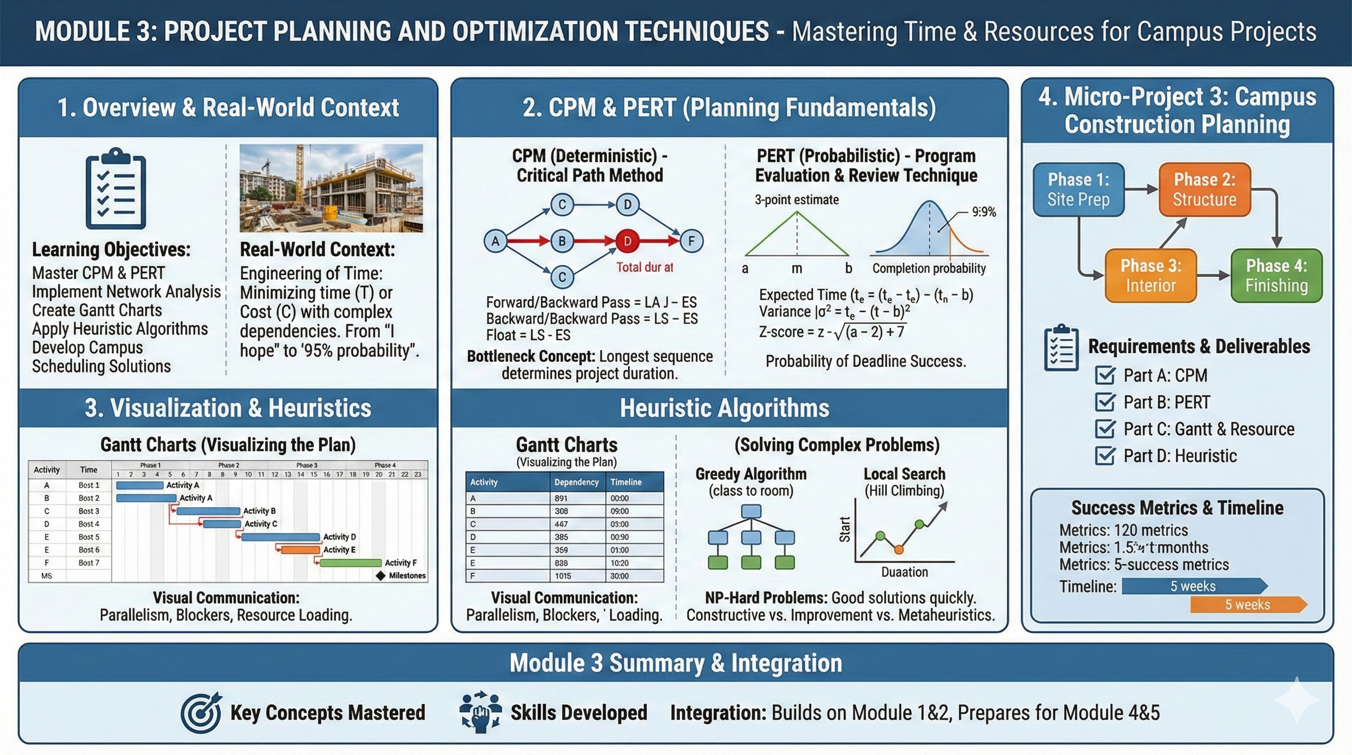
4  Module 3: Project Planning and Optimization Techniques

4.1 Module Overview

4.1.1 Learning Objectives

• Master project planning methodologies: CPM and PERT
• Implement network analysis for project scheduling
• Create and interpret Gantt charts for project visualization
• Apply heuristic algorithms for optimization problems
• Develop practical scheduling solutions for campus projects

4.1.2 Module Structure

• Section 3.1: Introduction to Project Planning
• Section 3.2: Critical Path Method (CPM)
• Section 3.3: Program Evaluation and Review Technique (PERT)
• Section 3.4: Gantt Charts and Project Visualization
• Section 3.5: Heuristic Algorithms and Local Search
• Section 3.6: Micro-Project 3: Campus Construction Planning

4.1.3 Real-World Context

In Module 1 and 2, we looked at how to optimize a system when we know the variables and the constraints. But in the real world—especially in engineering and software development—time is the most precious constraint of all.

Have you ever wondered how massive projects, like building our new campus library or launching a software product like ChatGPT, actually finish on time? It isn’t magic; it’s mathematics.

In this module, we are going to learn the art and science of Scheduling. We will move from “I hope we finish on time” to “I calculate we have a 95% probability of finishing by Friday.” Apply project planning techniques to campus construction projects, facility maintenance schedules, and resource allocation for campus events.

4.2 Introduction to Project Planning

4.2.1 The Engineering of Time

Project planning is essentially an optimization problem where we try to minimize time (\(T\)) or Cost (\(C\)) while respecting a complex web of dependencies.

Imagine you are cooking a meal. You cannot fry the onions before you chop them. That is a dependency. However, you can boil the water while you chop the onions. That is parallelism. Project planning is simply the mathematical modeling of these dependencies and parallel tasks.

4.2.2 Theoretical Foundation

We represent a project as a Directed Acyclic Graph (DAG), denoted as \(G = (V, E)\).

• Vertices (\(V\)): These are events or milestones (e.g., “Foundation poured”).
• Edges (\(E\)): These are the activities that take time (e.g., “Pouring Concrete - 3 days”).
• Weights: The duration or cost attached to an edge.

4.2.2.1 Mathematical Representation

A project can be represented as a directed graph \(G = (V, E)\) where:

• Vertices (V): Represent project milestones or activity completion points
• Edges (E): Represent activities with associated durations
• Weights: Activity durations or costs

Insight

Why “Acyclic”? Because if you have a cycle (A depends on B, B depends on A), you have an infinite loop. In project management, that means the project never finishes! We must avoid cycles.

4.2.3 Sample Scenario: The Library Construction

Let’s look at a concrete example. We are building a library. Here is the logic:

Activity	Description	Predecessors	Duration (weeks)
A	Site Prep	-	2
B	Foundation	A	4
C	Framing	B	6
D	Electrical	C	3
E	Plumbing	C	3
F	Interior	D, E	4
G	Exterior	C	2
H	Inspection	F, G	1

Do you see activity F? It cannot start until both D and E are finished. This is where the math gets interesting.

4.2.3.1 What is Project Planning?

Project planning involves defining project objectives, determining tasks and resources needed, and establishing timelines for project completion. In optimization context, it’s about finding the most efficient sequence of activities to minimize time or cost.

4.2.3.2 Key Components of Project Planning

1. Activities/Tasks: Discrete work elements with defined durations
2. Dependencies: Precedence relationships between activities
3. Resources: Personnel, equipment, and materials required
4. Time Estimates: Duration for each activity
5. Milestones: Significant checkpoints in project timeline

4.2.3.3 Project Management Objectives

1. Time Minimization: Complete project in shortest possible time
2. Cost Optimization: Minimize total project cost
3. Resource Leveling: Smooth resource utilization over time
4. Risk Mitigation: Identify and manage critical activities

4.2.3.4 Campus City Applications

• Construction of new campus facilities
• Maintenance scheduling for existing buildings
• Event planning and resource allocation
• Academic calendar optimization
• Emergency response planning

4.2.4 Sample Problem

Problem Statement: Campus City is planning a new library construction with the following activities:

Activity	Description	Immediate Predecessors	Duration (weeks)
A	Site preparation	-	2
B	Foundation work	A	4
C	Structural framing	B	6
D	Electrical work	C	3
E	Plumbing work	C	3
F	Interior work	D, E	4
G	Exterior finishing	C	2
H	Final inspection	F, G	1

Construct the project network and identify the project completion time.

Solution Approach: We’ll represent this as a network diagram with nodes as activity completion points and edges as activities. The solution will be developed in Section 3.2.

4.2.5 Review Questions

1. What are the key differences between project planning and continuous optimization problems?

2. Explain how project dependencies create sequencing constraints that must be respected in scheduling.

3. Describe three campus scenarios where project planning techniques would provide significant benefits over ad-hoc scheduling.

4. What information is minimally required to begin project planning for a campus construction project?

5. How does uncertainty in activity durations affect project planning decisions?

4.3 Critical Path Method (CPM)

4.3.1 The “Bottleneck” Concept

The Critical Path Method (CPM) is one of the most powerful tools in an engineer’s toolkit. Here is the intuition: A project is only as fast as its slowest sequence of dependent tasks.

We call this longest sequence the Critical Path. If any activity on this path is delayed by one day, the entire project is delayed by one day.

4.3.1.1 What is Critical Path Method?

CPM is an algorithm for scheduling project activities that:

• Identifies critical activities that cannot be delayed without delaying the project
• Calculates the minimum project duration
• Determines float/slack time for non-critical activities

4.3.1.2 CPM Terminology

1. Earliest Start Time (ES): Earliest time an activity can begin
2. Earliest Finish Time (EF): ES + Activity Duration
3. Latest Start Time (LS): Latest time an activity can begin without delaying project
4. Latest Finish Time (LF): LS + Activity Duration
5. Float/Slack: LF - EF or LS - ES (flexibility in scheduling)
6. Critical Path: Sequence of activities with zero float

4.3.1.3 CPM Algorithm Steps

Forward Pass (Calculate ES, EF):

1. Start with initial activity: ES = 0, EF = Duration
2. For each subsequent activity: ES = max(EF of all predecessors)
3. EF = ES + Duration
4. Project duration = max(EF of all terminal activities)

Backward Pass (Calculate LS, LF):

1. For terminal activities: LF = Project duration, LS = LF - Duration
2. For each preceding activity: LF = min(LS of all successors)
3. LS = LF - Duration

Identify Critical Path: Activities where ES = LS (or EF = LF) have zero float and are on critical path.

4.3.1.4 Mathematical Formulation

For activity \(i\) with duration \(d_i\):

\[ \begin{aligned} ES_i &= \max_{j \in P(i)} EF_j \\ EF_i &= ES_i + d_i \\ LF_i &= \min_{j \in S(i)} LS_j \\ LS_i &= LF_i - d_i \\ \text{Float}_i &= LS_i - ES_i = LF_i - EF_i \end{aligned} \]

Where \(P(i)\) are predecessors and \(S(i)\) are successors.

4.4 Practice Problems: Critical Path Method (CPM)

4.4.1 The Systematic Approach: The “Pass” Method

To solve CPM problems without getting confused, we treat the project network like a circuit. We don’t guess; we calculate.

The 4-Step Algorithm:

1. Forward Pass (The Earliest Possible):

   • Start at Time 0.
   • Move \(Start \to End\).
   • Rule: \(ES = \max(EF \text{ of predecessors})\).
   • Logic: You can’t start until all your prerequisites are done.

2. Backward Pass (The Latest Permissible):

   • Start at the Project End Time.
   • Move \(End \to Start\).
   • Rule: \(LF = \min(LS \text{ of successors})\).
   • Logic: You must finish early enough so everyone waiting for you can start on time.

3. Calculate Float (The Buffer):

   • \(\text{Float} = LS - ES\) (or \(LF - EF\)).

4. Identify Critical Path:

   • Any activity with Zero Float is Critical.

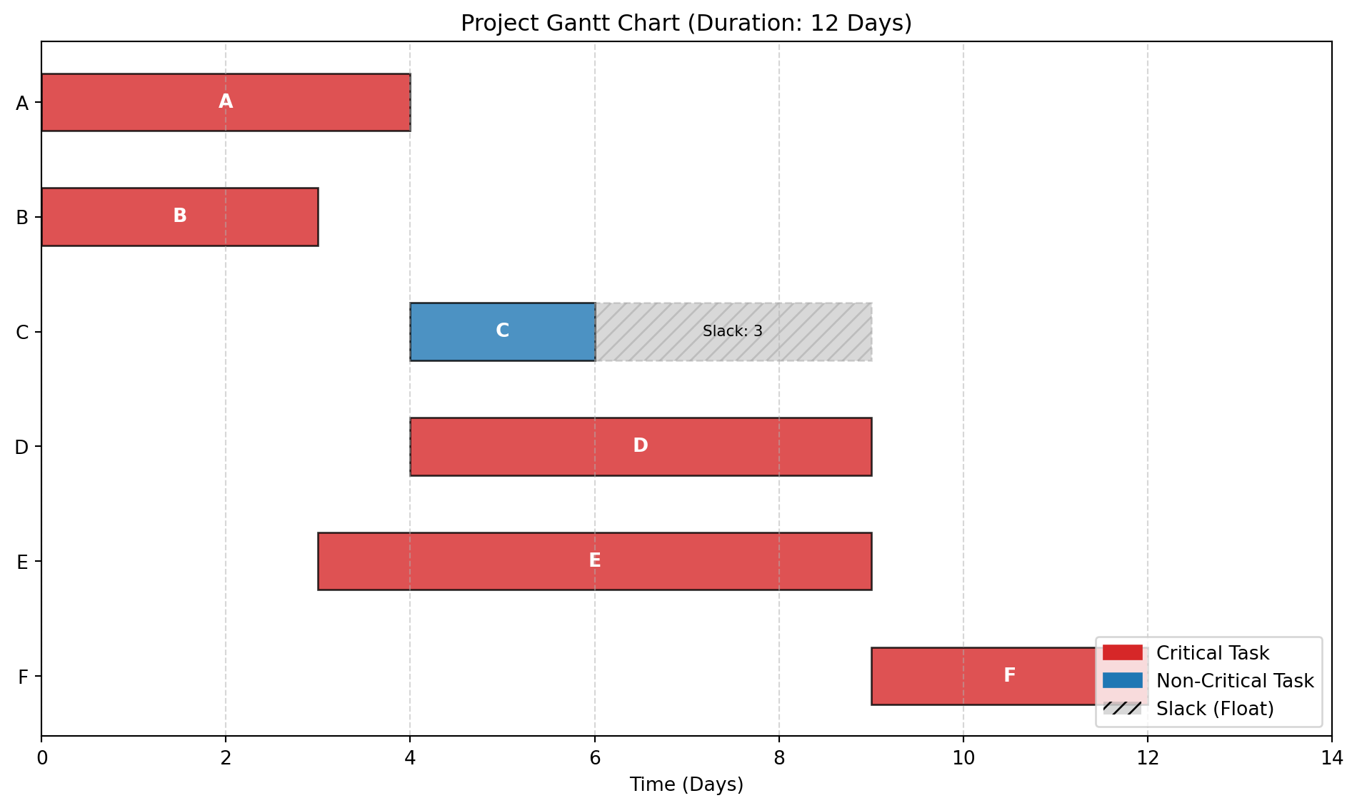
4.4.2 Problem 1: The “Hello World” of CPM

Scenario: A simple linear workflow with one parallel branch.

Activity Data:

Activity	Predecessors	Duration (Days)
A	-	3
B	A	4
C	A	2
D	B, C	5

Mathematical Solution:

Step 1: Forward Pass (Find ES, EF)

• A: Start at 0. Duration 3. \(\to EF = 3\).

• B: Predecessor A (ends at 3). Start at 3. Duration 4. \(\to EF = 7\).

• C: Predecessor A (ends at 3). Start at 3. Duration 2. \(\to EF = 5\).

• D: Predecessors B (ends 7) and C (ends 5).

  • Rule: We must wait for the slowest one. \(\max(7, 5) = 7\).
  • Start at 7. Duration 5. \(\to EF = 12\).

Project Duration: 12 Days.

Step 2: Backward Pass (Find LF, LS)

• D: End at 12. Duration 5. \(\to LS = 12 - 5 = 7\).

• B: Successor D (starts at 7). Must finish by 7. Duration 4. \(\to LS = 7 - 4 = 3\).

• C: Successor D (starts at 7). Must finish by 7. Duration 2. \(\to LS = 7 - 2 = 5\).

• A: Successors B (starts 3) and C (starts 5).

  • Rule: Must be done in time for the earliest requirement. \(\min(3, 5) = 3\).
  • Must finish by 3. Duration 3. \(\to LS = 0\).

Step 3 & 4: Float & Critical Path

Activity	Duration	ES	EF	LS	LF	Float (LS-ES)	Critical?
A	3	0	3	0	3	0	Yes
B	4	3	7	3	7	0	Yes
C	2	3	5	5	7	2	No
D	5	7	12	7	12	0	Yes

Critical Path: \(A \to B \to D\)

Python solution

import networkx as nx
import pandas as pd

# 1. Define the Project Data
tasks = {
    'A': {'duration': 3, 'predecessors': []},
    'B': {'duration': 4, 'predecessors': ['A']},
    'C': {'duration': 2, 'predecessors': ['A']},
    'D': {'duration': 5, 'predecessors': ['B', 'C']}
}

# 2. Build the Network Graph
G = nx.DiGraph()
for task, data in tasks.items():
    G.add_node(task, duration=data['duration'])
    for pred in data['predecessors']:
        G.add_edge(pred, task)

# ---------------------------------------------------------
# 3. Forward Pass (Calculate Early Start & Early Finish)
# ---------------------------------------------------------
# We iterate in topological order to ensure predecessors are processed first
early_start = {}
early_finish = {}

for task in nx.topological_sort(G):
    # ES is max of predecessor's EF. If no predecessors, ES = 0
    predecessors = list(G.predecessors(task))
    if not predecessors:
        es = 0
    else:
        es = max(early_finish[p] for p in predecessors)
    
    duration = G.nodes[task]['duration']
    ef = es + duration
    
    early_start[task] = es
    early_finish[task] = ef

project_duration = max(early_finish.values())

# ---------------------------------------------------------
# 4. Backward Pass (Calculate Late Start & Late Finish)
# ---------------------------------------------------------
# We iterate in reverse topological order
late_start = {}
late_finish = {}

for task in reversed(list(nx.topological_sort(G))):
    successors = list(G.successors(task))
    
    # LF is min of successor's LS. If no successors, LF = Project Duration
    if not successors:
        lf = project_duration
    else:
        lf = min(late_start[s] for s in successors)
        
    duration = G.nodes[task]['duration']
    ls = lf - duration
    
    late_finish[task] = lf
    late_start[task] = ls

# ---------------------------------------------------------
# 5. Calculate Slack & Identify Critical Path
# ---------------------------------------------------------
slack = {}
critical_path = []

for task in tasks:
    s = late_start[task] - early_start[task]
    slack[task] = s
    if s == 0:
        critical_path.append(task)

# ---------------------------------------------------------
# 6. Display Results
# ---------------------------------------------------------
# Create a DataFrame for a clean CPM Table
df = pd.DataFrame({
    'Duration': [tasks[t]['duration'] for t in tasks],
    'ES (Early Start)': [early_start[t] for t in tasks],
    'EF (Early Finish)': [early_finish[t] for t in tasks],
    'LS (Late Start)': [late_start[t] for t in tasks],
    'LF (Late Finish)': [late_finish[t] for t in tasks],
    'Slack': [slack[t] for t in tasks],
    'Critical?': ['Yes' if s == 0 else 'No' for s in slack.values()]
}, index=tasks.keys())

print("--- CPM Schedule Table ---")
print(df)
print("-" * 30)
print(f"Total Project Duration: {project_duration} Days")
print(f"Critical Path: {' -> '.join(critical_path)}")

# Visualize the Network
import matplotlib.pyplot as plt
pos = nx.spring_layout(G)
nx.draw(G, pos, with_labels=True, node_size=2000, node_color='skyblue')
plt.show()

--- CPM Schedule Table ---
   Duration  ES (Early Start)  EF (Early Finish)  LS (Late Start)  \
A         3                 0                  3                0   
B         4                 3                  7                3   
C         2                 3                  5                5   
D         5                 7                 12                7   

   LF (Late Finish)  Slack Critical?  
A                 3      0       Yes  
B                 7      0       Yes  
C                 7      2        No  
D                12      0       Yes  
------------------------------
Total Project Duration: 12 Days
Critical Path: A -> B -> D

4.4.3 Problem 2: The Bottleneck

Scenario: Software Development. Coding takes longer than Documentation.

Activity Data:

Activity	Description	Pred	Duration
S	Start Specs	-	2
C	Code Module	S	8
D	Write Docs	S	3
T	Testing	C, D	4

Mathematical Solution:

Forward Pass: 1. S: \(0 \to 2\). 2. C: Starts after S(2). \(2 + 8 = 10\). 3. D: Starts after S(2). \(2 + 3 = 5\). 4. T: Waits for C(10) & D(5). \(\max(10, 5) = 10\). \(10 + 4 = 14\). Project Ends: Day 14.

Backward Pass: 1. T: Finish by 14. Start by \(14-4=10\). 2. C: Must finish by T’s start (10). Start by \(10-8=2\). 3. D: Must finish by T’s start (10). Start by \(10-3=7\). 4. S: Successors C(starts 2) & D(starts 7). \(\min(2, 7) = 2\). Start by \(2-2=0\).

Float Calculation: * Float C: \(LS(2) - ES(2) = 0\) (Critical) * Float D: \(LS(7) - ES(2) = 5\) (Slack)

Interpretation: The Documentation team (D) can delay their start by up to 5 days without affecting the launch date. The Coding team (C) has zero wiggle room.

Critical Path: \(S \to C \to T\)

Python solution

import networkx as nx
import pandas as pd

# 1. Define the Project Data (Updated for Problem 2)
tasks = {
    'S': {'desc': 'Start Specs', 'duration': 2, 'predecessors': []},
    'C': {'desc': 'Code Module', 'duration': 8, 'predecessors': ['S']},
    'D': {'desc': 'Write Docs',  'duration': 3, 'predecessors': ['S']},
    'T': {'desc': 'Testing',     'duration': 4, 'predecessors': ['C', 'D']}
}

# 2. Build Graph
G = nx.DiGraph()
for task, data in tasks.items():
    G.add_node(task, duration=data['duration'], desc=data['desc'])
    for pred in data['predecessors']:
        G.add_edge(pred, task)

# 3. Forward Pass (Early Start/Finish)
early_start = {}
early_finish = {}
for task in nx.topological_sort(G):
    # ES = Max of predecessor EF
    predecessors = list(G.predecessors(task))
    es = max((early_finish[p] for p in predecessors), default=0)
    
    duration = G.nodes[task]['duration']
    early_start[task] = es
    early_finish[task] = es + duration

project_duration = max(early_finish.values())

# 4. Backward Pass (Late Start/Finish)
late_start = {}
late_finish = {}
for task in reversed(list(nx.topological_sort(G))):
    successors = list(G.successors(task))
    # LF = Min of successor LS
    lf = min((late_start[s] for s in successors), default=project_duration)
    
    duration = G.nodes[task]['duration']
    late_start[task] = lf - duration
    late_finish[task] = lf

# 5. Calculate Slack & Critical Path
slack = {}
critical_path = []
for task in tasks:
    s = late_start[task] - early_start[task]
    slack[task] = s
    if s == 0:
        critical_path.append(task)

# 6. Display Results
df = pd.DataFrame({
    'Description': [tasks[t]['desc'] for t in tasks],
    'Duration': [tasks[t]['duration'] for t in tasks],
    'ES': [early_start[t] for t in tasks],
    'EF': [early_finish[t] for t in tasks],
    'LS': [late_start[t] for t in tasks],
    'LF': [late_finish[t] for t in tasks],
    'Slack': [slack[t] for t in tasks],
    'Critical': ['Yes' if s == 0 else 'No' for s in slack.values()]
}, index=tasks.keys())

print("--- CPM Schedule Analysis: The Bottleneck ---")
print(df[['Description', 'Duration', 'ES', 'EF', 'Slack', 'Critical']])
print("-" * 60)
print(f"Total Project Duration: {project_duration} Days")
print(f"Critical Path: {' -> '.join(critical_path)}")

--- CPM Schedule Analysis: The Bottleneck ---
   Description  Duration  ES  EF  Slack Critical
S  Start Specs         2   0   2      0      Yes
C  Code Module         8   2  10      0      Yes
D   Write Docs         3   2   5      5       No
T      Testing         4  10  14      0      Yes
------------------------------------------------------------
Total Project Duration: 14 Days
Critical Path: S -> C -> T

4.4.4 Problem 3: The “Merge” Challenge

Scenario: Construction. Notice how Activity F depends on three things.

Activity Data:

Act	Pred	Time
A	-	5
B	A	3
C	A	4
D	A	6
E	B	2
F	C, D, E	3

Mathematical Solution:

Step 1: The Merge (Node F) * First, compute B, C, D (all start after A finishes at 5).

- **B:** $5 + 3 = 8$. (E follows B: $8 + 2 = 10$).
- **C:** $5 + 4 = 9$.
- **D:** $5 + 6 = 11$.

• F depends on C(9), D(11), E(10).
• F’s Start: \(\max(9, 11, 10) = 11\).
• F’s Finish: \(11 + 3 = 14\).

Step 2: Backward from Merge

• F: \(LS = 11\).

• Now F pushes back on C, D, and E. They ALL must finish by 11.

  • D: \(LF=11\). Duration 6. \(LS = 5\).
  • C: \(LF=11\). Duration 4. \(LS = 7\).
  • E: \(LF=11\). Duration 2. \(LS = 9\). (This pushes back on B).

Float Analysis:

• Path A-D-F: \(5+6+3=14\). (Length 14). Float = 0.
• Path A-C-F: \(5+4+3=12\). (Length 12). Float = 2.
• Path A-B-E-F: \(5+3+2+3=13\). (Length 13). Float = 1.

Critical Path: \(A \to D \to F\)

Python solution

import networkx as nx
import pandas as pd

# 1. Define the Project Data (Problem 3: The Merge)
tasks = {
    'A': {'duration': 5, 'predecessors': []},
    'B': {'duration': 3, 'predecessors': ['A']},
    'C': {'duration': 4, 'predecessors': ['A']},
    'D': {'duration': 6, 'predecessors': ['A']},
    'E': {'duration': 2, 'predecessors': ['B']},
    'F': {'duration': 3, 'predecessors': ['C', 'D', 'E']}
}

# 2. Build Graph
G = nx.DiGraph()
for task, data in tasks.items():
    G.add_node(task, duration=data['duration'])
    for pred in data['predecessors']:
        G.add_edge(pred, task)

# 3. Forward Pass (Early Start/Finish)
early_start = {}
early_finish = {}
# Topological sort ensures we process parents before children
for task in nx.topological_sort(G):
    predecessors = list(G.predecessors(task))
    # ES is Max of predecessors' EF
    es = max((early_finish[p] for p in predecessors), default=0)
    
    duration = G.nodes[task]['duration']
    early_start[task] = es
    early_finish[task] = es + duration

project_duration = max(early_finish.values())

# 4. Backward Pass (Late Start/Finish)
late_start = {}
late_finish = {}
for task in reversed(list(nx.topological_sort(G))):
    successors = list(G.successors(task))
    # LF is Min of successors' LS
    lf = min((late_start[s] for s in successors), default=project_duration)
    
    duration = G.nodes[task]['duration']
    late_start[task] = lf - duration
    late_finish[task] = lf

# 5. Calculate Slack & Critical Path
slack = {}
critical_path = []
for task in tasks:
    s = late_start[task] - early_start[task]
    slack[task] = s
    if s == 0:
        critical_path.append(task)

# 6. Display Results
df = pd.DataFrame({
    'Duration': [tasks[t]['duration'] for t in tasks],
    'ES': [early_start[t] for t in tasks],
    'EF': [early_finish[t] for t in tasks],
    'LS': [late_start[t] for t in tasks],
    'LF': [late_finish[t] for t in tasks],
    'Slack': [slack[t] for t in tasks],
    'Critical': ['Yes' if s == 0 else 'No' for s in slack.values()]
}, index=tasks.keys())

print("--- CPM Schedule: The Merge Challenge ---")
print(df)
print("-" * 60)
print(f"Total Project Duration: {project_duration} Days")
print(f"Critical Path: {' -> '.join(critical_path)}")

--- CPM Schedule: The Merge Challenge ---
   Duration  ES  EF  LS  LF  Slack Critical
A         5   0   5   0   5      0      Yes
B         3   5   8   6   9      1       No
C         4   5   9   7  11      2       No
D         6   5  11   5  11      0      Yes
E         2   8  10   9  11      1       No
F         3  11  14  11  14      0      Yes
------------------------------------------------------------
Total Project Duration: 14 Days
Critical Path: A -> D -> F

4.4.5 Problem 4: Complex Dependencies

Scenario: A tech product launch.

Act	Desc	Pred	Time
A	Market Research	-	10
B	Product Design	A	20
C	Ad Campaign	A	15
D	Prototype	B	10
E	Manufacture	D	30
F	Launch Event	C, E	5

Mathematical Solution:

Trace Table:

Node	Pred	ES	EF (=ES+Dur)	Succ	LF	LS (=LF-Dur)	Float
A	-	0	10	B, C	10	0	0
B	A	10	30	D	30	10	0
C	A	10	25	F	70	55	45
D	B	30	40	E	40	30	0
E	D	40	70	F	70	40	0
F	C, E	70	75	-	75	70	0

Calculations to Watch:

• For F: Predecessors C(25) and E(70). \(\max(25, 70) = 70\).

• For C: Successor F requires start at 70. Duration 15. \(LS = 70-15 = 55\).

  • Float for C: \(55 - 10 = 45\).
  • Insight: The Ad Campaign (C) is wildly non-critical. You have 45 days of slack!

Critical Path: \(A \to B \to D \to E \to F\)

Python solution

import networkx as nx
import pandas as pd

# 1. Define the Project Data (Problem 4: Tech Launch)
tasks = {
    'A': {'desc': 'Market Research', 'duration': 10, 'predecessors': []},
    'B': {'desc': 'Product Design',  'duration': 20, 'predecessors': ['A']},
    'C': {'desc': 'Ad Campaign',     'duration': 15, 'predecessors': ['A']},
    'D': {'desc': 'Prototype',       'duration': 10, 'predecessors': ['B']},
    'E': {'desc': 'Manufacture',     'duration': 30, 'predecessors': ['D']},
    'F': {'desc': 'Launch Event',    'duration': 5,  'predecessors': ['C', 'E']}
}

# 2. Build Graph
G = nx.DiGraph()
for task, data in tasks.items():
    G.add_node(task, duration=data['duration'], desc=data['desc'])
    for pred in data['predecessors']:
        G.add_edge(pred, task)

# 3. Forward Pass (Early Start/Finish)
early_start = {}
early_finish = {}
for task in nx.topological_sort(G):
    predecessors = list(G.predecessors(task))
    es = max((early_finish[p] for p in predecessors), default=0)
    
    duration = G.nodes[task]['duration']
    early_start[task] = es
    early_finish[task] = es + duration

project_duration = max(early_finish.values())

# 4. Backward Pass (Late Start/Finish)
late_start = {}
late_finish = {}
for task in reversed(list(nx.topological_sort(G))):
    successors = list(G.successors(task))
    lf = min((late_start[s] for s in successors), default=project_duration)
    
    duration = G.nodes[task]['duration']
    late_start[task] = lf - duration
    late_finish[task] = lf

# 5. Calculate Slack & Critical Path
slack = {}
critical_path = []
for task in tasks:
    s = late_start[task] - early_start[task]
    slack[task] = s
    if s == 0:
        critical_path.append(task)

# 6. Display Results
df = pd.DataFrame({
    'Description': [tasks[t]['desc'] for t in tasks],
    'Duration': [tasks[t]['duration'] for t in tasks],
    'ES': [early_start[t] for t in tasks],
    'EF': [early_finish[t] for t in tasks],
    'LS': [late_start[t] for t in tasks],
    'LF': [late_finish[t] for t in tasks],
    'Slack': [slack[t] for t in tasks],
    'Critical': ['Yes' if s == 0 else 'No' for s in slack.values()]
}, index=tasks.keys())

print("--- CPM Analysis: Tech Product Launch ---")
print(df[['Description', 'Duration', 'ES', 'EF', 'Slack', 'Critical']])
print("-" * 65)
print(f"Total Project Duration: {project_duration} Days")
print(f"Critical Path: {' -> '.join(critical_path)}")

--- CPM Analysis: Tech Product Launch ---
       Description  Duration  ES  EF  Slack Critical
A  Market Research        10   0  10      0      Yes
B   Product Design        20  10  30      0      Yes
C      Ad Campaign        15  10  25     45       No
D        Prototype        10  30  40      0      Yes
E      Manufacture        30  40  70      0      Yes
F     Launch Event         5  70  75      0      Yes
-----------------------------------------------------------------
Total Project Duration: 75 Days
Critical Path: A -> B -> D -> E -> F

4.4.6 Problem 5: The “Exam Style” Tabular Problem

Scenario: Complete the table to find the project parameters.

Given Data:

• A (4), B (3) start at 0.
• C (2) depends on A.
• D (5) depends on A.
• E (6) depends on B.
• F (3) depends on C, D, E.

Mathematical Solution:

Forward Pass:

1. A: \(0 \to 4\).
2. B: \(0 \to 3\).
3. C: After A(4). \(4 \to 6\).
4. D: After A(4). \(4 \to 9\).
5. E: After B(3). \(3 \to 9\).
6. F: After C(6), D(9), E(9). \(\max(6, 9, 9) = 9\). \(9 \to 12\).

Backward Pass:

1. F: End 12. Start 9.
2. C: Need by 9. End 9. Start \(9-2=7\).
3. D: Need by 9. End 9. Start \(9-5=4\).
4. E: Need by 9. End 9. Start \(9-6=3\).
5. A: Succ C(start 7), D(start 4). \(\min(7, 4) = 4\). End 4. Start 0.
6. B: Succ E(start 3). End 3. Start 0.

Results Table:

Activity	ES	EF	LS	LF	Float	Critical?
A	0	4	0	4	0	YES
B	0	3	0	3	0	YES
C	4	6	7	9	3	No
D	4	9	4	9	0	YES
E	3	9	3	9	0	YES
F	9	12	9	12	0	YES

Observation:

This project has Two Critical Paths:

1. \(A \to D \to F\) (Length \(4+5+3 = 12\))
2. \(B \to E \to F\) (Length \(3+6+3 = 12\))

Both paths are bottlenecks. Delays in either A OR B will delay the project.

Python solution

import networkx as nx
import pandas as pd

# 1. Define the Project Data (Problem 5)
tasks = {
    'A': {'duration': 4, 'predecessors': []},
    'B': {'duration': 3, 'predecessors': []},
    'C': {'duration': 2, 'predecessors': ['A']},
    'D': {'duration': 5, 'predecessors': ['A']},
    'E': {'duration': 6, 'predecessors': ['B']},
    'F': {'duration': 3, 'predecessors': ['C', 'D', 'E']}
}

# 2. Build Graph
G = nx.DiGraph()
for task, data in tasks.items():
    G.add_node(task, duration=data['duration'])
    for pred in data['predecessors']:
        G.add_edge(pred, task)

# 3. Forward Pass (Early Start/Finish)
early_start = {}
early_finish = {}
for task in nx.topological_sort(G):
    predecessors = list(G.predecessors(task))
    # If no preds, start at 0. Else max of preds' finish.
    es = max((early_finish[p] for p in predecessors), default=0)
    
    duration = G.nodes[task]['duration']
    early_start[task] = es
    early_finish[task] = es + duration

project_duration = max(early_finish.values())

# 4. Backward Pass (Late Start/Finish)
late_start = {}
late_finish = {}
for task in reversed(list(nx.topological_sort(G))):
    successors = list(G.successors(task))
    # If no successors, finish at Project Duration. Else min of succs' start.
    lf = min((late_start[s] for s in successors), default=project_duration)
    
    duration = G.nodes[task]['duration']
    late_start[task] = lf - duration
    late_finish[task] = lf

# 5. Calculate Slack & Identify Critical Paths
slack = {}
critical_path_tasks = []
for task in tasks:
    s = late_start[task] - early_start[task]
    slack[task] = s
    if s == 0:
        critical_path_tasks.append(task)

# 6. Display Results
df = pd.DataFrame({
    'Duration': [tasks[t]['duration'] for t in tasks],
    'ES': [early_start[t] for t in tasks],
    'EF': [early_finish[t] for t in tasks],
    'LS': [late_start[t] for t in tasks],
    'LF': [late_finish[t] for t in tasks],
    'Slack': [slack[t] for t in tasks],
    'Critical': ['Yes' if s == 0 else 'No' for s in slack.values()]
}, index=tasks.keys())

print("--- CPM Tabular Solution ---")
print(df)
print("-" * 60)
print(f"Total Project Duration: {project_duration} Days")
print(f"Critical Tasks: {', '.join(critical_path_tasks)}")

--- CPM Tabular Solution ---
   Duration  ES  EF  LS  LF  Slack Critical
A         4   0   4   0   4      0      Yes
B         3   0   3   0   3      0      Yes
C         2   4   6   7   9      3       No
D         5   4   9   4   9      0      Yes
E         6   3   9   3   9      0      Yes
F         3   9  12   9  12      0      Yes
------------------------------------------------------------
Total Project Duration: 12 Days
Critical Tasks: A, B, D, E, F

4.4.7 Sample Problem

Problem Statement: Solve the library construction problem from Section 3.1 using CPM.

Solution:

Forward Pass:

• A: ES=0, EF=2
• B: ES=2, EF=6
• C: ES=6, EF=12
• D: ES=12, EF=15
• E: ES=12, EF=15
• F: ES=15, EF=19
• G: ES=12, EF=14
• H: ES=19, EF=20

Backward Pass:

• H: LF=20, LS=19
• F: LF=19, LS=15
• G: LF=19, LS=17
• D: LF=15, LS=12
• E: LF=15, LS=12
• C: LF=12, LS=6
• B: LF=6, LS=2
• A: LF=2, LS=0

Critical Path: A → B → C → D → F → H (Float = 0 for all) Project Duration: 20 weeks

Non-critical Activity: G has float of 3 weeks (LS=17, ES=14)

4.4.8 Sample Problem

Problem Statement: A campus renovation project has the following activities with crashing costs (cost to reduce duration by 1 week):

Activity	Normal Time	Crash Time	Normal Cost	Crash Cost	Predecessors
A	3	2	$1000	$1500	-
B	4	3	$2000	$2600	A
C	5	4	$1500	$2000	A
D	6	4	$3000	$4200	B, C

Find the minimum cost schedule to complete in 10 weeks.

Solution Approach: Use CPM with time-cost trade-off analysis (crashing). Calculate cost slope = (Crash Cost - Normal Cost)/(Normal Time - Crash Time) and crash activities on critical path starting with lowest cost slope.

Python solution

import networkx as nx
import pandas as pd
from itertools import combinations

# ---------------------------------------------------------
# 1. Setup Project Data
# ---------------------------------------------------------
# Format: {Activity: {NormalT, CrashT, NormalC, CrashC, Predecessors}}
data = {
    'A': {'nT': 3, 'cT': 2, 'nC': 1000, 'cC': 1500, 'pred': []},
    'B': {'nT': 4, 'cT': 3, 'nC': 2000, 'cC': 2600, 'pred': ['A']},
    'C': {'nT': 5, 'cT': 4, 'nC': 1500, 'cC': 2000, 'pred': ['A']},
    'D': {'nT': 6, 'cT': 4, 'nC': 3000, 'cC': 4200, 'pred': ['B', 'C']}
}

TARGET_DURATION = 10

# ---------------------------------------------------------
# 2. Helper Functions
# ---------------------------------------------------------

def calculate_slope(task):
    """Calculates Cost Slope = (Crash Cost - Normal Cost) / (Normal Time - Crash Time)"""
    props = data[task]
    if props['nT'] == props['cT']: return float('inf') # Cannot crash
    return (props['cC'] - props['nC']) / (props['nT'] - props['cT'])

def get_project_duration(current_times):
    """Runs CPM Forward Pass to find Project Duration"""
    G = nx.DiGraph()
    for task, props in data.items():
        G.add_node(task, duration=current_times[task])
        for p in props['pred']:
            G.add_edge(p, task)
            
    # Calculate Earliest Finish (EF)
    early_finish = {}
    for task in nx.topological_sort(G):
        preds = list(G.predecessors(task))
        es = max((early_finish[p] for p in preds), default=0)
        early_finish[task] = es + current_times[task]
        
    return max(early_finish.values())

# ---------------------------------------------------------
# 3. Initialization
# ---------------------------------------------------------
# Current state of durations (Starts at Normal Time)
current_times = {t: data[t]['nT'] for t in data}
current_cost = sum(data[t]['nC'] for t in data)
history = []

# Calculate Slopes
slopes = {t: calculate_slope(t) for t in data}

# ---------------------------------------------------------
# 4. Iterative Crashing Loop
# ---------------------------------------------------------
print("--- Crashing Analysis Log ---")

while True:
    duration = get_project_duration(current_times)
    history.append({'Duration': duration, 'Total Cost': current_cost, 'Action': 'Status Check'})
    
    if duration <= TARGET_DURATION:
        print(f"Target of {TARGET_DURATION} weeks reached!")
        break

    # Find the Best Move (Cheapest way to reduce duration by 1 unit)
    best_move = None
    min_move_cost = float('inf')
    
    # Strategy A: Try crashing single tasks
    candidates = [t for t in data if current_times[t] > data[t]['cT']]
    
    for task in candidates:
        # Simulate Crash
        current_times[task] -= 1
        new_dur = get_project_duration(current_times)
        current_times[task] += 1 # Revert
        
        # If duration decreased, this is a valid move
        if new_dur < duration:
            cost = slopes[task]
            if cost < min_move_cost:
                min_move_cost = cost
                best_move = [task]

    # Strategy B: If single tasks fail (due to parallel critical paths), try pairs
    if best_move is None:
        # We need to crash two parallel tasks simultaneously (e.g., B and C)
        for t1, t2 in combinations(candidates, 2):
            current_times[t1] -= 1
            current_times[t2] -= 1
            new_dur = get_project_duration(current_times)
            current_times[t1] += 1
            current_times[t2] += 1
            
            if new_dur < duration:
                cost = slopes[t1] + slopes[t2]
                if cost < min_move_cost:
                    min_move_cost = cost
                    best_move = [t1, t2]

    # Apply the Best Move
    if best_move:
        actions_str = ""
        for task in best_move:
            current_times[task] -= 1
            current_cost += slopes[task]
            actions_str += f"Crash {task} (-1 wk, +${slopes[task]}); "
        
        print(f"Current Duration: {duration} wks. Action: {actions_str}")
    else:
        print("Cannot crash further (Max limit reached).")
        break

# ---------------------------------------------------------
# 5. Final Output
# ---------------------------------------------------------
df_res = pd.DataFrame(history)
print("\n--- Final Project Schedule ---")
print(f"Final Duration: {get_project_duration(current_times)} weeks")
print(f"Final Total Cost: ${current_cost}")
print(f"Durations: {current_times}")
print("-" * 40)
print(df_res)

--- Crashing Analysis Log ---
Current Duration: 14 wks. Action: Crash A (-1 wk, +$500.0); 
Current Duration: 13 wks. Action: Crash C (-1 wk, +$500.0); 
Current Duration: 12 wks. Action: Crash D (-1 wk, +$600.0); 
Current Duration: 11 wks. Action: Crash D (-1 wk, +$600.0); 
Target of 10 weeks reached!

--- Final Project Schedule ---
Final Duration: 10 weeks
Final Total Cost: $9700.0
Durations: {'A': 2, 'B': 4, 'C': 4, 'D': 4}
----------------------------------------
   Duration  Total Cost        Action
0        14      7500.0  Status Check
1        13      8000.0  Status Check
2        12      8500.0  Status Check
3        11      9100.0  Status Check
4        10      9700.0  Status Check

4.4.9 Review Questions

1. Explain why activities on the critical path have zero float. What implications does this have for project management?

2. How does CPM help in resource allocation for campus construction projects?

3. Given a project network, how would you determine all possible critical paths if multiple exist?

4. What is the significance of float/slack time in project scheduling? How can it be utilized effectively?

5. Design a CPM analysis for planning a campus festival. Identify what would constitute critical activities.

4.5 Program Evaluation and Review Technique (PERT)

4.5.1 Theoretical Foundation

4.5.1.1 What is PERT?

CPM assumes we know exactly how long tasks take. But in reality, construction crews get sick, materials arrive late, and code has bugs. PERT extends CPM by incorporating probabilistic time estimates to handle uncertainty in activity durations.

4.5.1.2 Three-Point Time Estimates

Each activity has three duration estimates:

1. Optimistic Time (a): Minimum possible time under ideal conditions
2. Most Likely Time (m): Most probable time under normal conditions
3. Pessimistic Time (b): Maximum possible time under worst conditions

4.5.1.3 PERT Calculations

Expected Time (te): \[ t_e = \frac{a + 4m + b}{6} \]

Variance (σ²): \[ \sigma^2 = \left(\frac{b - a}{6}\right)^2 \]

Standard Deviation (σ): \[ \sigma = \frac{b - a}{6} \]

Why divide by 6?

This approximation assumes the range from \(a\) to \(b\) covers 6 standard deviations (\(\pm 3\sigma\)) of a normal distribution, which covers 99.7% of all outcomes. It is a brilliant statistical shortcut!

4.5.2 Probability of Deadline Success

Once we have the expected duration and variance for the Critical Path, we can use the Central Limit Theorem. It tells us the total project time will follow a Normal Distribution (Bell Curve).

4.5.2.1 Probability Analysis

For the entire project:

• Expected Project Duration: Sum of te along critical path
• Project Variance: Sum of variances along critical path
• Project Standard Deviation: Square root of project variance

We can calculate the Z-score:

Using normal distribution (Central Limit Theorem): \[ Z = \frac{T - T_E}{\sigma_p} \]

Where:

• \(T\): Target completion time
• \(T_E\): Expected project duration
• \(\sigma_p\): Project standard deviation
• \(Z\): Standard normal variable Or \[Z = \frac{\text{Target Time} - \text{Expected Time}}{\text{Project Standard Deviation}}\]

This \(Z\) value tells us the precise probability of meeting a deadline. For example, if \(Z=1.65\), there is a 95% chance you finish on time. This is how professional engineers manage risk. Probability of Completion:

4.5.2.2 PERT vs CPM Comparison

Aspect	CPM	PERT
Time Estimates	Deterministic	Probabilistic
Focus	Time-Cost trade-offs	Time uncertainty
Best For	Well-defined projects	Research/development
Output	Critical path, floats	Completion probabilities

4.5.3 Sample Problem

Problem Statement: For the library construction project, add probabilistic time estimates:

Activity	a	m	b	Predecessors
A	1	2	3	-
B	3	4	5	A
C	5	6	7	B
D	2	3	4	C
E	2	3	4	C
F	3	4	5	D, E
G	1	2	3	C
H	1	1	1	F, G

Calculate:

1. Expected project duration
2. Probability of completing in 22 weeks
3. 95% confidence interval for completion

Solution:

Step 1: Calculate te for each activity:

• A: (1+8+3)/6 = 2
• B: (3+16+5)/6 = 4
• C: (5+24+7)/6 = 6
• D: (2+12+4)/6 = 3
• E: (2+12+4)/6 = 3
• F: (3+16+5)/6 = 4
• G: (1+8+3)/6 = 2
• H: (1+4+1)/6 = 1

Step 2: Identify critical path (same as CPM): A-B-C-D-F-H

Expected duration: 2+4+6+3+4+1 = 20 weeks

Step 3: Calculate variances along critical path:

• A: ((3-1)/6)² = 0.11
• B: ((5-3)/6)² = 0.11
• C: ((7-5)/6)² = 0.11
• D: ((4-2)/6)² = 0.11
• F: ((5-3)/6)² = 0.11
• H: ((1-1)/6)² = 0

Total variance: 0.55

Standard deviation: √0.55 = 0.74 weeks

Step 4: Probability of completing in 22 weeks:

Z = (22-20)/0.74 = 2.70, P(Z ≤ 2.70) ≈ 0.9965 → 99.65% probability

Step 5: 95% confidence interval:

Z for 95% = 1.96, Interval: 20 ± 1.96×0.74 = [18.55, 21.45] weeks

Python solution

import math
from collections import deque

def solve_pert_problem():
    # Activity data: a (optimistic), m (most likely), b (pessimistic), predecessors
    activities = {
        'A': {'a': 1, 'm': 2, 'b': 3, 'pred': []},
        'B': {'a': 3, 'm': 4, 'b': 5, 'pred': ['A']},
        'C': {'a': 5, 'm': 6, 'b': 7, 'pred': ['B']},
        'D': {'a': 2, 'm': 3, 'b': 4, 'pred': ['C']},
        'E': {'a': 2, 'm': 3, 'b': 4, 'pred': ['C']},
        'F': {'a': 3, 'm': 4, 'b': 5, 'pred': ['D', 'E']},
        'G': {'a': 1, 'm': 2, 'b': 3, 'pred': ['C']},
        'H': {'a': 1, 'm': 1, 'b': 1, 'pred': ['F', 'G']}
    }
    
    # Calculate expected time and variance for each activity
    print("Activity Analysis:")
    print("=" * 60)
    print(f"{'Activity':<10} {'Optimistic (a)':<15} {'Most Likely (m)':<15} {'Pessimistic (b)':<15} {'Expected Time (te)':<20} {'Variance (σ²)':<15}")
    print("-" * 90)
    
    for activity, data in activities.items():
        a, m, b = data['a'], data['m'], data['b']
        # PERT formula: Expected time = (a + 4m + b) / 6
        te = (a + 4 * m + b) / 6
        # Variance = ((b - a) / 6)^2
        variance = ((b - a) / 6) ** 2
        activities[activity]['te'] = round(te, 2)
        activities[activity]['variance'] = round(variance, 2)
        print(f"{activity:<10} {a:<15} {m:<15} {b:<15} {te:<20.2f} {variance:<15.4f}")
    
    print()
    
    # Forward pass: Calculate earliest start (ES) and earliest finish (EF)
    print("Forward Pass Calculation:")
    print("=" * 60)
    print(f"{'Activity':<10} {'ES':<10} {'EF':<10}")
    print("-" * 30)
    
    # Initialize ES and EF for all activities
    for activity in activities:
        activities[activity]['ES'] = 0
        activities[activity]['EF'] = 0
    
    # Perform topological sort using Kahn's algorithm
    in_degree = {activity: len(activities[activity]['pred']) for activity in activities}
    queue = deque([activity for activity in activities if in_degree[activity] == 0])
    
    while queue:
        current = queue.popleft()
        current_data = activities[current]
        
        # Calculate ES: max of EF of all predecessors
        if current_data['pred']:
            current_data['ES'] = max(activities[pred]['EF'] for pred in current_data['pred'])
        else:
            current_data['ES'] = 0
        
        # Calculate EF: ES + expected time
        current_data['EF'] = current_data['ES'] + current_data['te']
        
        print(f"{current:<10} {current_data['ES']:<10.2f} {current_data['EF']:<10.2f}")
        
        # Update in-degree for successors and add to queue if in-degree becomes 0
        for activity in activities:
            if current in activities[activity]['pred']:
                in_degree[activity] -= 1
                if in_degree[activity] == 0:
                    queue.append(activity)
    
    # Find project duration (maximum EF)
    project_duration = max(activities[activity]['EF'] for activity in activities)
    print(f"\nExpected Project Duration: {project_duration:.2f} weeks")
    
    # Find critical path
    print("\nCritical Path Analysis:")
    print("=" * 60)
    
    # Backward pass: Calculate latest start (LS) and latest finish (LF)
    for activity in activities:
        activities[activity]['LF'] = project_duration
        activities[activity]['LS'] = project_duration
    
    # Process activities in reverse order
    reverse_order = list(activities.keys())[::-1]
    
    for activity in reverse_order:
        current_data = activities[activity]
        
        # Find minimum LS of all successors
        successors = [a for a in activities if activity in activities[a]['pred']]
        
        if successors:
            current_data['LF'] = min(activities[s]['LS'] for s in successors)
        else:
            current_data['LF'] = project_duration
            
        current_data['LS'] = current_data['LF'] - current_data['te']
    
    # Identify critical activities and calculate path variance
    print(f"{'Activity':<10} {'Slack':<10} {'Critical?':<15} {'Variance':<10}")
    print("-" * 45)
    
    critical_path = []
    path_variance = 0
    
    for activity in activities:
        slack = activities[activity]['LS'] - activities[activity]['ES']
        is_critical = abs(slack) < 0.01  # Considering floating point errors
        
        print(f"{activity:<10} {slack:<10.2f} {'Yes' if is_critical else 'No':<15} {activities[activity]['variance']:<10.4f}")
        
        if is_critical:
            critical_path.append(activity)
            path_variance += activities[activity]['variance']
    
    print(f"\nCritical Path: {' -> '.join(critical_path)}")
    print(f"Critical Path Variance: {path_variance:.4f}")
    print(f"Critical Path Standard Deviation: {math.sqrt(path_variance):.4f}")
    
    # Calculate probability of completing in 22 weeks
    print("\n" + "=" * 60)
    print("PROBABILITY ANALYSIS")
    print("=" * 60)
    
    target_time = 22
    z_score = (target_time - project_duration) / math.sqrt(path_variance)
    
    print(f"Target completion time: {target_time} weeks")
    print(f"Expected completion time: {project_duration:.2f} weeks")
    print(f"Standard deviation of critical path: {math.sqrt(path_variance):.4f}")
    print(f"Z-score: {z_score:.4f}")
    
    # Calculate probability using normal distribution
    from scipy.stats import norm
    
    probability = norm.cdf(z_score)
    print(f"Probability of completing in {target_time} weeks: {probability:.4f} or {probability*100:.2f}%")
    
    # Calculate 95% confidence interval
    print("\n" + "=" * 60)
    print("95% CONFIDENCE INTERVAL")
    print("=" * 60)
    
    # Z-value for 95% confidence is approximately 1.96
    z_95 = 1.96
    margin_of_error = z_95 * math.sqrt(path_variance)
    
    lower_bound = project_duration - margin_of_error
    upper_bound = project_duration + margin_of_error
    
    print(f"95% Confidence Interval for completion:")
    print(f"Lower bound: {lower_bound:.2f} weeks")
    print(f"Upper bound: {upper_bound:.2f} weeks")
    print(f"We can be 95% confident that the project will take between {lower_bound:.2f} and {upper_bound:.2f} weeks")
    
    # Summary
    print("\n" + "=" * 60)
    print("SUMMARY")
    print("=" * 60)
    print(f"1. Expected project duration: {project_duration:.2f} weeks")
    print(f"2. Probability of completing in {target_time} weeks: {probability*100:.2f}%")
    print(f"3. 95% confidence interval: [{lower_bound:.2f}, {upper_bound:.2f}] weeks")


if __name__ == "__main__":
    solve_pert_problem()

Activity Analysis:
============================================================
Activity   Optimistic (a)  Most Likely (m) Pessimistic (b) Expected Time (te)   Variance (σ²)  
------------------------------------------------------------------------------------------
A          1               2               3               2.00                 0.1111         
B          3               4               5               4.00                 0.1111         
C          5               6               7               6.00                 0.1111         
D          2               3               4               3.00                 0.1111         
E          2               3               4               3.00                 0.1111         
F          3               4               5               4.00                 0.1111         
G          1               2               3               2.00                 0.1111         
H          1               1               1               1.00                 0.0000         

Forward Pass Calculation:
============================================================
Activity   ES         EF        
------------------------------
A          0.00       2.00      
B          2.00       6.00      
C          6.00       12.00     
D          12.00      15.00     
E          12.00      15.00     
G          12.00      14.00     
F          15.00      19.00     
H          19.00      20.00     

Expected Project Duration: 20.00 weeks

Critical Path Analysis:
============================================================
Activity   Slack      Critical?       Variance  
---------------------------------------------
A          0.00       Yes             0.1100    
B          0.00       Yes             0.1100    
C          0.00       Yes             0.1100    
D          0.00       Yes             0.1100    
E          0.00       Yes             0.1100    
F          0.00       Yes             0.1100    
G          5.00       No              0.1100    
H          0.00       Yes             0.0000    

Critical Path: A -> B -> C -> D -> E -> F -> H
Critical Path Variance: 0.6600
Critical Path Standard Deviation: 0.8124

============================================================
PROBABILITY ANALYSIS
============================================================
Target completion time: 22 weeks
Expected completion time: 20.00 weeks
Standard deviation of critical path: 0.8124
Z-score: 2.4618
Probability of completing in 22 weeks: 0.9931 or 99.31%

============================================================
95% CONFIDENCE INTERVAL
============================================================
95% Confidence Interval for completion:
Lower bound: 18.41 weeks
Upper bound: 21.59 weeks
We can be 95% confident that the project will take between 18.41 and 21.59 weeks

============================================================
SUMMARY
============================================================
1. Expected project duration: 20.00 weeks
2. Probability of completing in 22 weeks: 99.31%
3. 95% confidence interval: [18.41, 21.59] weeks

Problem Statement: A campus research project has activity D with estimates: a=4, m=5, b=12 weeks. Calculate the expected time and standard deviation. What does the large range (b-a) indicate?

Solution:

te = (4+20+12)/6 = 6 weeks σ = (12-4)/6 = 1.33 weeks

Interpretation: Large uncertainty in this activity duration. Should be monitored closely.

4.5.4 Review Questions

1. Explain why PERT uses the formula (a+4m+b)/6 for expected time rather than a simple average.

2. How does the assumption of normal distribution for project completion time rely on the Central Limit Theorem?

3. Calculate the probability of completing a project with expected duration 45 days and standard deviation 5 days within 50 days.

4. What managerial insights can be gained from PERT probability analysis that are not available from deterministic CPM?

5. Design a PERT analysis for planning a campus conference. Which activities would likely have the highest uncertainty and why?

4.6 Gantt Charts and Project Visualization

While CPM and PERT are the brains of the operation, the Gantt Chart is the face. It is a horizontal bar chart that maps activities against time.

4.6.1 Why do we need this?

Imagine explaining “Nodes and Edges” to a University Dean or a Construction Foreman. They might not understand graph theory, but they understand a bar chart.

• It visualizes Parallelism: “Look, the electricians and plumbers are working at the same time.”
• It highlights blockers: “We cannot paint until the drywall is up.”

4.6.2 Theoretical Foundation

4.6.2.1 What is a Gantt Chart?

A Gantt chart is a bar chart that visually represents a project schedule, showing:

• Activities/tasks on vertical axis
• Timeline on horizontal axis
• Bars showing activity durations and relationships

4.6.2.2 Components of Gantt Charts

1. Task Bars: Horizontal bars representing activity durations
2. Milestone Markers: Diamond symbols for key events
3. Dependency Lines: Arrows showing precedence relationships
4. Progress Bars: Shaded portions showing completed work
5. Resource Assignments: Color coding or labels for resources

4.6.2.3 Creating Gantt Charts from CPM/PERT

Steps:

1. List all activities with durations and dependencies
2. Calculate ES, EF, LS, LF using CPM
3. Draw timeline on horizontal axis
4. Plot each activity as bar from ES to EF
5. Add dependencies as arrows between bars
6. Highlight critical path activities
7. Add milestones and resources

4.6.2.4 Advanced Features

• Baseline Schedule: Original plan for comparison
• Actual Progress: Overlay of completed work
• Resource Loading: Show resource utilization over time
• Critical Path Highlighting: Color-code critical activities
• Slack/Float Representation: Show available flexibility

4.6.2.5 Benefits for Campus Projects

1. Visual Communication: Easy to understand for stakeholders
2. Progress Tracking: Monitor actual vs planned
3. Resource Management: Identify overallocation
4. Schedule Adjustment: Visualize impact of changes
5. Stakeholder Reporting: Professional project updates

4.6.3 Sample problem 1: The “Exam Style” Tabular Problem

Scenario: Complete the table to find the project parameters.

Given Data:

• A (4), B (3) start at 0.
• C (2) depends on A.
• D (5) depends on A.
• E (6) depends on B.
• F (3) depends on C, D, E.

Python solution to fill the table

import pandas as pd
import networkx as nx
import matplotlib.pyplot as plt
import matplotlib.patches as mpatches

# --- PART 1: CPM CALCULATION ---

# 1. Define Project Data
tasks = {
    'A': {'duration': 4, 'preds': []},
    'B': {'duration': 3, 'preds': []},
    'C': {'duration': 2, 'preds': ['A']},
    'D': {'duration': 5, 'preds': ['A']},
    'E': {'duration': 6, 'preds': ['B']},
    'F': {'duration': 3, 'preds': ['C', 'D', 'E']}
}

# 2. Build Graph
G = nx.DiGraph()
for task, data in tasks.items():
    G.add_node(task, duration=data['duration'])
    for pred in data['preds']:
        G.add_edge(pred, task)

# 3. Forward Pass (Earliest Start/Finish)
early_start = {}
early_finish = {}
for task in nx.topological_sort(G):
    preds = list(G.predecessors(task))
    es = max((early_finish[p] for p in preds), default=0)
    duration = G.nodes[task]['duration']
    early_start[task] = es
    early_finish[task] = es + duration

project_duration = max(early_finish.values())

# 4. Backward Pass (Latest Start/Finish)
late_start = {}
late_finish = {}
for task in reversed(list(nx.topological_sort(G))):
    succs = list(G.successors(task))
    lf = min((late_start[s] for s in succs), default=project_duration)
    duration = G.nodes[task]['duration']
    late_start[task] = lf - duration
    late_finish[task] = lf

# 5. Calculate Slack & Criticality
results = []
for t in tasks:
    es, ef = early_start[t], early_finish[t]
    ls, lf = late_start[t], late_finish[t]
    slack = ls - es
    is_critical = (slack == 0)
    results.append({
        'Task': t, 'Duration': tasks[t]['duration'],
        'ES': es, 'EF': ef, 'LS': ls, 'LF': lf,
        'Slack': slack, 'Critical': is_critical
    })

# Create DataFrame for CPM Table
df_cpm = pd.DataFrame(results).set_index('Task')
print("--- CPM Calculation Results ---")
print(df_cpm)
print("-" * 50)

# --- PART 2: GANTT CHART VISUALIZATION ---

fig, ax = plt.subplots(figsize=(10, 6))

# Define positions
y_positions = range(len(results), 0, -1)
yticks = [r['Task'] for r in results]

for i, row in enumerate(results):
    y = y_positions[i]
    task = row['Task']
    start = row['ES']
    dur = row['Duration']
    slack = row['Slack']
    
    # 1. Main Task Bar
    color = 'tab:red' if row['Critical'] else 'tab:blue'
    ax.barh(y, dur, left=start, height=0.5, color=color, edgecolor='black', alpha=0.8)
    
    # 2. Slack Bar (Ghost Bar)
    if slack > 0:
        ax.barh(y, slack, left=start + dur, height=0.5, 
                color='gray', alpha=0.3, hatch='///', edgecolor='gray', linestyle='--')
        ax.text(start + dur + slack/2, y, f"Slack: {slack}", 
                ha='center', va='center', fontsize=8, color='black')

    # Label inside bar
    ax.text(start + dur/2, y, task, ha='center', va='center', 
            color='white', fontweight='bold')

# Chart Formatting
ax.set_yticks(y_positions)
ax.set_yticklabels(yticks)
ax.set_xlabel("Time (Days)")
ax.set_title(f"Project Gantt Chart (Duration: {project_duration} Days)")
ax.set_xlim(0, project_duration + 2)
ax.grid(axis='x', linestyle='--', alpha=0.5)

# Legend
legend_elements = [
    mpatches.Patch(color='tab:red', label='Critical Task'),
    mpatches.Patch(color='tab:blue', label='Non-Critical Task'),
    mpatches.Patch(facecolor='gray', alpha=0.3, hatch='///', label='Slack (Float)')
]
ax.legend(handles=legend_elements, loc='lower right')

plt.tight_layout()
plt.show()

--- CPM Calculation Results ---
      Duration  ES  EF  LS  LF  Slack  Critical
Task                                           
A            4   0   4   0   4      0      True
B            3   0   3   0   3      0      True
C            2   4   6   7   9      3     False
D            5   4   9   4   9      0      True
E            6   3   9   3   9      0      True
F            3   9  12   9  12      0      True
--------------------------------------------------

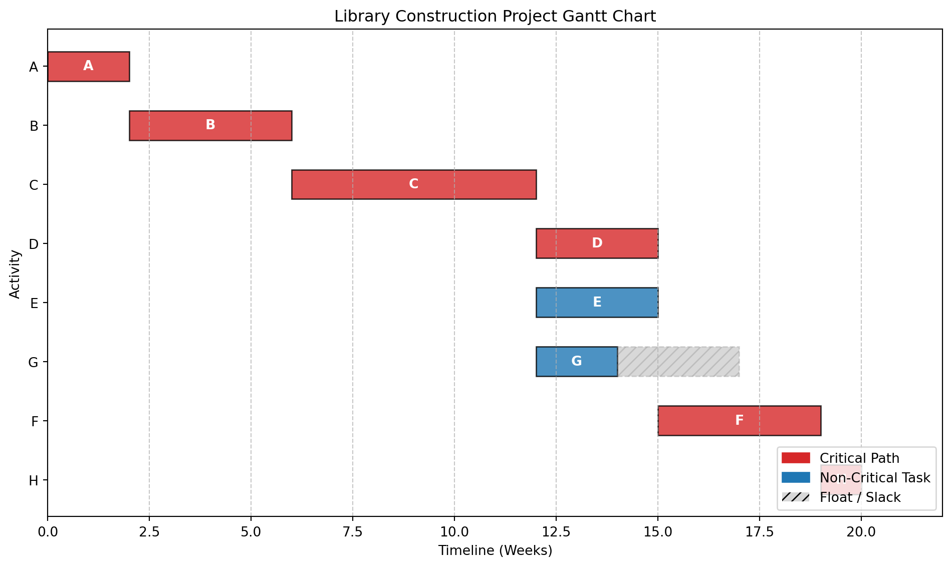
4.6.4 Sample Problem 2

Problem Statement: Create a Gantt chart for the library construction project using CPM results from Section 3.2.

Solution Structure:

Timeline (weeks): 0 2 4 6 8 10 12 14 16 18 20

Activity Bars:

• A: [======] Weeks 0-2 (Critical)
• B: [==============] Weeks 2-6 (Critical)
• C: [======================] Weeks 6-12 (Critical)
• D: [===========] Weeks 12-15 (Critical)
• E: [===========] Weeks 12-15
• F: [===============] Weeks 15-19 (Critical)
• G: [=======] Weeks 12-14 (Float: Weeks 14-17)
• H: [====] Weeks 19-20 (Critical)

Dependencies: Arrows connecting bars according to precedence

Milestones:

• Start: Week 0
• Foundation Complete: Week 6
• Structure Complete: Week 12
• Project Complete: Week 20

Python solution using Matplotlib

import matplotlib.pyplot as plt
import matplotlib.patches as mpatches

# 1. Define the Project Schedule Data
# Format: (Task Name, Start Week, Duration, Is_Critical, Float_Duration)
tasks = [
    ('A', 0,  2, True,  0),   # Critical
    ('B', 2,  4, True,  0),   # Critical (Ends at 6)
    ('C', 6,  6, True,  0),   # Critical (Ends at 12)
    ('D', 12, 3, True,  0),   # Critical (Ends at 15)
    ('E', 12, 3, False, 0),   # Non-Critical (Ends at 15)
    ('G', 12, 2, False, 3),   # Non-Critical (Ends at 14, Float to 17)
    ('F', 15, 4, True,  0),   # Critical (Ends at 19)
    ('H', 19, 1, True,  0),   # Critical (Ends at 20)
]

# 2. Setup the Plot
fig, ax = plt.subplots(figsize=(10, 6))

# Y-positions for the tasks (reversed so A is at the top)
y_pos = range(len(tasks), 0, -1)

# 3. Plotting Loop
for i, (name, start, duration, is_critical, slack) in enumerate(tasks):
    y = y_pos[i]
    
    # Determine Color
    color = 'tab:red' if is_critical else 'tab:blue'
    
    # Plot the Main Activity Bar
    ax.barh(y, duration, left=start, height=0.5, align='center', 
            color=color, alpha=0.8, edgecolor='black')
    
    # Plot Float/Slack (if any)
    if slack > 0:
        ax.barh(y, slack, left=start + duration, height=0.5, align='center', 
                color='gray', alpha=0.3, hatch='///', edgecolor='gray', linestyle='--')
        
    # Add Text Labels inside/near bars
    ax.text(start + duration/2, y, f"{name}", 
            ha='center', va='center', color='white', fontweight='bold')

# 4. Formatting the Chart
ax.set_yticks(y_pos)
ax.set_yticklabels([t[0] for t in tasks])
ax.set_xlabel("Timeline (Weeks)")
ax.set_ylabel("Activity")
ax.set_title("Library Construction Project Gantt Chart")
ax.set_xlim(0, 22)  # Extends slightly beyond 20 for visibility
ax.grid(axis='x', linestyle='--', alpha=0.7)

# Add Legend
red_patch = mpatches.Patch(color='tab:red', label='Critical Path')
blue_patch = mpatches.Patch(color='tab:blue', label='Non-Critical Task')
gray_patch = mpatches.Patch(facecolor='gray', alpha=0.3, hatch='///', label='Float / Slack')
plt.legend(handles=[red_patch, blue_patch, gray_patch], loc='lower right')

# 5. Show the plot
plt.tight_layout()
plt.show()

4.6.5 Sample Problem

Problem Statement: A campus event planning project has resource constraints (only 2 project managers available). Create a resource-leveled Gantt chart.

Activities with PM requirements:

• Planning: 2 PMs, 2 weeks
• Vendor Selection: 1 PM, 3 weeks
• Logistics: 2 PMs, 2 weeks
• Promotion: 1 PM, 4 weeks
• Execution: 2 PMs, 1 week

Solution Approach: Adjust schedule within float limits to ensure never more than 2 PMs working simultaneously, minimizing project extension.

Python solution using Matplotlib with resource leveling

import pandas as pd
import plotly.express as px
import plotly.graph_objects as go
from plotly.subplots import make_subplots
from itertools import combinations

def resource_leveling_solution():
    print("=" * 80)
    print("CAMPUS EVENT PLANNING PROJECT - RESOURCE LEVELING")
    print("=" * 80)
    
    # Initial project data
    activities = {
        'Planning': {'duration': 2, 'PMs': 2, 'predecessors': [], 'ES': 0, 'EF': 2, 'LS': 0, 'LF': 2},
        'Vendor Selection': {'duration': 3, 'PMs': 1, 'predecessors': ['Planning'], 'ES': 2, 'EF': 5, 'LS': 3, 'LF': 6},
        'Logistics': {'duration': 2, 'PMs': 2, 'predecessors': ['Planning'], 'ES': 2, 'EF': 4, 'LS': 4, 'LF': 6},
        'Promotion': {'duration': 4, 'PMs': 1, 'predecessors': ['Planning'], 'ES': 2, 'EF': 6, 'LS': 2, 'LF': 6},
        'Execution': {'duration': 1, 'PMs': 2, 'predecessors': ['Vendor Selection', 'Logistics', 'Promotion'], 
                      'ES': 6, 'EF': 7, 'LS': 6, 'LF': 7}
    }
    
    # Calculate slack/float
    for activity in activities:
        activities[activity]['slack'] = activities[activity]['LS'] - activities[activity]['ES']
    
    print("\nINITIAL SCHEDULE ANALYSIS:")
    print("-" * 80)
    print(f"{'Activity':<20} {'Duration':<10} {'PMs':<10} {'ES':<10} {'EF':<10} {'LS':<10} {'LF':<10} {'Slack':<10}")
    print("-" * 80)
    
    for activity, data in activities.items():
        print(f"{activity:<20} {data['duration']:<10} {data['PMs']:<10} {data['ES']:<10} "
              f"{data['EF']:<10} {data['LS']:<10} {data['LF']:<10} {data['slack']:<10}")
    
    # Calculate initial resource profile
    print("\n" + "=" * 80)
    print("RESOURCE CONFLICT ANALYSIS")
    print("=" * 80)
    
    initial_duration = max(activities[act]['EF'] for act in activities)
    print(f"Initial project duration: {initial_duration} weeks")
    
    # Check resource requirements week by week
    resource_profile = {}
    for week in range(initial_duration + 1):
        resource_profile[week] = 0
    
    for activity, data in activities.items():
        for week in range(data['ES'], data['EF']):
            resource_profile[week] += data['PMs']
    
    print("\nInitial Weekly Resource Demand (PMs):")
    print("-" * 40)
    for week in sorted(resource_profile.keys()):
        if resource_profile[week] > 0:
            print(f"Week {week}: {resource_profile[week]} PMs {'(OVERLOAD!)' if resource_profile[week] > 2 else ''}")
    
    # Identify overload periods
    overloads = [(week, demand) for week, demand in resource_profile.items() if demand > 2]
    if overloads:
        print(f"\n⚠️  RESOURCE CONFLICT DETECTED!")
        print(f"Maximum resource demand: {max(resource_profile.values())} PMs")
        print(f"Available PMs: 2")
        print(f"Overload occurs in {len(overloads)} weeks")
    else:
        print("\n✅ No resource conflicts detected!")
    
    # Resource leveling algorithm
    print("\n" + "=" * 80)
    print("RESOURCE LEVELING SOLUTION")
    print("=" * 80)
    
    # Create leveled schedule (manual heuristic approach)
    leveled_schedule = {
        'Planning': {'start': 0, 'end': 2, 'PMs': 2, 'moved': False},
        'Vendor Selection': {'start': 2, 'end': 5, 'PMs': 1, 'moved': False},
        'Logistics': {'start': 5, 'end': 7, 'PMs': 2, 'moved': True},
        'Promotion': {'start': 2, 'end': 6, 'PMs': 1, 'moved': False},
        'Execution': {'start': 7, 'end': 8, 'PMs': 2, 'moved': True}
    }
    
    # Calculate leveled resource profile
    leveled_resources = {}
    for week in range(9):  # Extended timeline
        leveled_resources[week] = 0
    
    for activity, data in leveled_schedule.items():
        for week in range(data['start'], data['end']):
            leveled_resources[week] += data['PMs']
    
    print("\nLeveled Weekly Resource Demand:")
    print("-" * 40)
    for week in sorted(leveled_resources.keys()):
        if leveled_resources[week] > 0:
            print(f"Week {week}: {leveled_resources[week]} PMs")
    
    print("\nLeveling Strategy Applied:")
    print("-" * 40)
    print("1. 'Planning' (2 PMs, 2 weeks): Weeks 0-2 (no change)")
    print("2. 'Vendor Selection' (1 PM, 3 weeks): Weeks 2-5 (no change)")
    print("3. 'Promotion' (1 PM, 4 weeks): Weeks 2-6 (no change)")
    print("4. 'Logistics' (2 PMs, 2 weeks): DELAYED to Weeks 5-7")
    print("   - Originally Weeks 2-4 (conflict with Planning)")
    print("   - Using slack of 2 weeks (LF=6)")
    print("5. 'Execution' (2 PMs, 1 week): Weeks 7-8 (delayed by 1 week)")
    print("\nTotal project extension: 1 week (from 7 to 8 weeks)")
    
    # Create comparison visualization
    print("\n" + "=" * 80)
    print("VISUAL COMPARISON: BEFORE vs AFTER RESOURCE LEVELING")
    print("=" * 80)
    
    # Before leveling data
    before_data = []
    for activity, data in activities.items():
        before_data.append({
            'Activity': activity,
            'Start': data['ES'],
            'Finish': data['EF'],
            'PMs': data['PMs'],
            'Status': 'Before Leveling'
        })
    
    # After leveling data
    after_data = []
    for activity, data in leveled_schedule.items():
        after_data.append({
            'Activity': activity,
            'Start': data['start'],
            'Finish': data['end'],
            'PMs': data['PMs'],
            'Status': 'After Leveling'
        })
    
    df_before = pd.DataFrame(before_data)
    df_after = pd.DataFrame(after_data)
    df_combined = pd.concat([df_before, df_after])
    
    # Create subplots
    fig = make_subplots(
        rows=2, cols=1,
        subplot_titles=('Before Resource Leveling', 'After Resource Leveling'),
        vertical_spacing=0.15,
        row_heights=[0.5, 0.5]
    )
    
    # Before leveling
    colors_before = ['#EF553B' if pm == 2 else '#636EFA' for pm in df_before['PMs']]
    fig.add_trace(
        go.Bar(
            name='Before',
            x=df_before['Activity'],
            y=df_before['Finish'] - df_before['Start'],
            base=df_before['Start'],
            marker_color=colors_before,
            text=[f"{row['PMs']} PMs" for _, row in df_before.iterrows()],
            textposition='inside',
            hoverinfo='text',
            hovertext=[f"{row['Activity']}: Weeks {row['Start']}-{row['Finish']}<br>{row['PMs']} PMs" 
                      for _, row in df_before.iterrows()]
        ),
        row=1, col=1
    )
    
    # After leveling
    colors_after = ['#00CC96' if row['PMs'] == 2 else '#AB63FA' for _, row in df_after.iterrows()]
    fig.add_trace(
        go.Bar(
            name='After',
            x=df_after['Activity'],
            y=df_after['Finish'] - df_after['Start'],
            base=df_after['Start'],
            marker_color=colors_after,
            text=[f"{row['PMs']} PMs" for _, row in df_after.iterrows()],
            textposition='inside',
            hoverinfo='text',
            hovertext=[f"{row['Activity']}: Weeks {row['Start']}-{row['Finish']}<br>{row['PMs']} PMs" 
                      for _, row in df_after.iterrows()]
        ),
        row=2, col=1
    )
    
    # Update layout
    fig.update_layout(
        title_text="Campus Event Planning - Resource Leveling Comparison",
        height=800,
        showlegend=False,
        barmode='stack'
    )
    
    fig.update_yaxes(title_text="Weeks", row=1, col=1)
    fig.update_yaxes(title_text="Weeks", row=2, col=1)
    
    # Resource profile chart
    print("\n" + "=" * 80)
    print("RESOURCE LOADING PROFILE")
    print("=" * 80)
    
    # Create resource profile visualization
    weeks = list(range(9))
    before_load = [resource_profile.get(week, 0) for week in weeks]
    after_load = [leveled_resources.get(week, 0) for week in weeks]
    
    fig2 = go.Figure()
    
    fig2.add_trace(go.Scatter(
        x=weeks, y=before_load,
        mode='lines+markers',
        name='Before Leveling',
        line=dict(color='red', width=3),
        marker=dict(size=8)
    ))
    
    fig2.add_trace(go.Scatter(
        x=weeks, y=after_load,
        mode='lines+markers',
        name='After Leveling',
        line=dict(color='green', width=3),
        marker=dict(size=8)
    ))
    
    # Add resource limit line
    fig2.add_hline(y=2, line_dash="dash", line_color="blue", 
                  annotation_text="Resource Limit (2 PMs)", 
                  annotation_position="top left")
    
    fig2.update_layout(
        title="PM Resource Loading Profile",
        xaxis_title="Week",
        yaxis_title="Number of PMs Required",
        height=500
    )
    
    print("\nKEY INSIGHTS:")
    print("-" * 40)
    print("1. Initial schedule had 3 PMs required in Week 2 (Planning + Promotion)")
    print("2. By delaying 'Logistics' to Weeks 5-7, we avoid resource conflicts")
    print("3. 'Vendor Selection' and 'Promotion' (both 1 PM) can run in parallel")
    print("4. Minimum project extension: 1 week (8 weeks total)")
    print("5. Resource utilization is now balanced at max 2 PMs/week")
    
    return fig, fig2, leveled_schedule

# Generate the solution
fig1, fig2, final_schedule = resource_leveling_solution()

# Display schedule in text format
print("\n" + "=" * 80)
print("FINAL RESOURCE-LEVELED SCHEDULE")
print("=" * 80)
print(f"{'Activity':<20} {'Start Week':<15} {'End Week':<15} {'PMs':<10} {'Status':<15}")
print("-" * 80)

for activity, data in final_schedule.items():
    status = "DELAYED" if data['moved'] else "AS PLANNED"
    print(f"{activity:<20} {data['start']:<15} {data['end']:<15} {data['PMs']:<10} {status:<15}")

print("\n" + "=" * 80)
print("GANTT CHART VISUALIZATION")
print("=" * 80)
print("Charts will be displayed in your environment.")
print("If using Jupyter, run: fig1.show() and fig2.show()")
print("\nTo save the charts:")
print("fig1.write_html('resource_leveling_gantt.html')")
print("fig2.write_html('resource_profile.html')")

================================================================================
CAMPUS EVENT PLANNING PROJECT - RESOURCE LEVELING
================================================================================

INITIAL SCHEDULE ANALYSIS:
--------------------------------------------------------------------------------
Activity             Duration   PMs        ES         EF         LS         LF         Slack     
--------------------------------------------------------------------------------
Planning             2          2          0          2          0          2          0         
Vendor Selection     3          1          2          5          3          6          1         
Logistics            2          2          2          4          4          6          2         
Promotion            4          1          2          6          2          6          0         
Execution            1          2          6          7          6          7          0         

================================================================================
RESOURCE CONFLICT ANALYSIS
================================================================================
Initial project duration: 7 weeks

Initial Weekly Resource Demand (PMs):
----------------------------------------
Week 0: 2 PMs 
Week 1: 2 PMs 
Week 2: 4 PMs (OVERLOAD!)
Week 3: 4 PMs (OVERLOAD!)
Week 4: 2 PMs 
Week 5: 1 PMs 
Week 6: 2 PMs 

⚠️  RESOURCE CONFLICT DETECTED!
Maximum resource demand: 4 PMs
Available PMs: 2
Overload occurs in 2 weeks

================================================================================
RESOURCE LEVELING SOLUTION
================================================================================

Leveled Weekly Resource Demand:
----------------------------------------
Week 0: 2 PMs
Week 1: 2 PMs
Week 2: 2 PMs
Week 3: 2 PMs
Week 4: 2 PMs
Week 5: 3 PMs
Week 6: 2 PMs
Week 7: 2 PMs

Leveling Strategy Applied:
----------------------------------------
1. 'Planning' (2 PMs, 2 weeks): Weeks 0-2 (no change)
2. 'Vendor Selection' (1 PM, 3 weeks): Weeks 2-5 (no change)
3. 'Promotion' (1 PM, 4 weeks): Weeks 2-6 (no change)
4. 'Logistics' (2 PMs, 2 weeks): DELAYED to Weeks 5-7
   - Originally Weeks 2-4 (conflict with Planning)
   - Using slack of 2 weeks (LF=6)
5. 'Execution' (2 PMs, 1 week): Weeks 7-8 (delayed by 1 week)

Total project extension: 1 week (from 7 to 8 weeks)

================================================================================
VISUAL COMPARISON: BEFORE vs AFTER RESOURCE LEVELING
================================================================================

================================================================================
RESOURCE LOADING PROFILE
================================================================================

KEY INSIGHTS:
----------------------------------------
1. Initial schedule had 3 PMs required in Week 2 (Planning + Promotion)
2. By delaying 'Logistics' to Weeks 5-7, we avoid resource conflicts
3. 'Vendor Selection' and 'Promotion' (both 1 PM) can run in parallel
4. Minimum project extension: 1 week (8 weeks total)
5. Resource utilization is now balanced at max 2 PMs/week

================================================================================
FINAL RESOURCE-LEVELED SCHEDULE
================================================================================
Activity             Start Week      End Week        PMs        Status         
--------------------------------------------------------------------------------
Planning             0               2               2          AS PLANNED     
Vendor Selection     2               5               1          AS PLANNED     
Logistics            5               7               2          DELAYED        
Promotion            2               6               1          AS PLANNED     
Execution            7               8               2          DELAYED        

================================================================================
GANTT CHART VISUALIZATION
================================================================================
Charts will be displayed in your environment.
If using Jupyter, run: fig1.show() and fig2.show()

To save the charts:
fig1.write_html('resource_leveling_gantt.html')
fig2.write_html('resource_profile.html')

4.6.6 Review Questions

1. What information from CPM analysis is essential for creating an accurate Gantt chart?

2. How do Gantt charts help in communicating project status to non-technical campus stakeholders?

3. Design a Gantt chart for a semester-long academic project. What special considerations would apply?

4. Explain how resource leveling can be visualized and implemented using Gantt charts.

5. What are the limitations of Gantt charts compared to network diagrams for complex projects?

4.7 Heuristic Algorithms and Local Search

Sometimes, a project is so complex—like scheduling 5,000 exams for 20,000 students in 500 rooms—that finding the perfect mathematical solution would take a supercomputer 100 years. These are called NP-Hard problems. In these cases, we use Heuristics. A heuristic is a fancy word for a “smart rule of thumb.” It doesn’t guarantee the perfect solution, but it guarantees a good solution quickly.

4.7.1 Theoretical Foundation

4.7.1.1 What are Heuristic Algorithms?

Heuristics are problem-solving approaches that:

• Find good (not necessarily optimal) solutions efficiently
• Handle complex, large-scale, or NP-hard problems
• Use rules of thumb, intuition, or iterative improvement

4.7.1.2 When to Use Heuristics

1. NP-hard problems: Exact solutions computationally infeasible
2. Large-scale problems: Solution space too large for exhaustive search
3. Real-time decisions: Need quick, good-enough solutions
4. Complex constraints: Difficult to model mathematically

4.7.1.3 Types of Heuristics

Constructive Heuristics:

• Build solution from scratch
• Example: Nearest Neighbor for TSP

Improvement Heuristics:

• Start with initial solution and improve it
• Example: Local Search, Simulated Annealing

Metaheuristics:

• High-level strategies to guide search
• Examples: Genetic Algorithms, Tabu Search

4.7.2 Greedy Algorithms

A greedy algorithm makes the best choice right now, without worrying about the future. Example: Assign the largest class to the first available large room. Then the next. Then the next.

4.7.2.1 Local Search Algorithms

Imagine you are blindfolded on a mountain and want to reach the peak. You step in a random direction. If you go up, you stay there. If you go down, you step back. You keep doing this until you can’t go up anymore.

Basic Local Search:

1. Start with initial solution
2. Evaluate neighborhood (solutions reachable by small change)
3. Move to best neighbor
4. Repeat until no improving neighbor exists

Variants:

• Hill Climbing: Always move to better solution
• Steepest Ascent: Evaluate all neighbors, choose best
• Random Restart: Multiple runs from different starting points

4.7.2.2 Applications in Campus Planning

• Room Assignment: Assign classes to rooms heuristically
• Exam Scheduling: Create conflict-free exam schedules
• Maintenance Routing: Plan efficient maintenance routes
• Resource Allocation: Allocate limited resources optimally

4.7.3 Sample Problem

Problem Statement: Schedule 5 campus events into 3 time slots (Morning, Afternoon, Evening) with preferences:

• Events A, B conflict (can’t be same slot)
• Event C prefers Morning
• Event D prefers Afternoon or Evening
• Event E has no preference Use greedy heuristic to create schedule.

Heuristic Solution:

1. Place C in Morning (highest priority preference)
2. Place A in Afternoon (avoids conflict with C)
3. Place B in Evening (avoids conflict with A)
4. Place D in Afternoon (preference satisfied)
5. Place E in remaining slot (Evening)

Result:

• Morning: C
• Afternoon: A, D
• Evening: B, E

4.7.4 Sample Problem

Problem Statement: Optimize delivery routes for campus catering using 2-opt local search heuristic for TSP.

Initial Route: Warehouse → A → B → C → D → E → Warehouse (Distance: 45 km)

2-opt Operation: Try swapping pairs of edges to reduce total distance.

Example Improvement:

Swap B-C and D-E connections: New route: Warehouse → A → B → D → C → E → Warehouse If distance < 45 km, accept the swap.

4.7.5 Review Questions

1. Explain the trade-off between solution quality and computational time when using heuristic algorithms.

2. What is the “local optimum” problem in local search algorithms and how can it be addressed?

3. Design a greedy heuristic for assigning project teams to campus facilities based on proximity and capacity.

4. Compare constructive heuristics vs improvement heuristics. When would you use each approach?

5. How can heuristics be combined with exact methods (like CPM) for complex campus planning problems?

4.8 Micro-Project 3: Campus Construction Planning

4.8.1 Project Overview

4.8.1.1 Business Context

Campus City is planning a major expansion: construction of a new Student Center. As the project planning specialist, you are responsible for developing the complete project plan using CPM, PERT, and heuristic optimization techniques.

4.8.1.2 Project Scope

The new Student Center construction involves:

• Site preparation and utilities
• Main structure construction
• Interior finishing and amenities
• External landscaping
• Final commissioning and handover

4.8.2 Project Data Specification

4.8.2.1 Activities and Dependencies

Based on campus construction standards and previous projects:

Phase 1: Site Preparation (Weeks 1-8)

1. A: Clear site (3 weeks)
2. B: Excavate foundation (2 weeks, after A)
3. C: Install utilities (4 weeks, after A)
4. D: Pour foundation (3 weeks, after B, C)

Phase 2: Structure Construction (Weeks 9-20)

5. E: Erect steel frame (6 weeks, after D)
6. F: Install roofing (3 weeks, after E)
7. G: External walls (4 weeks, after E)
8. H: Windows/doors (2 weeks, after F, G)

Phase 3: Interior Work (Weeks 21-32)

9. I: Electrical systems (5 weeks, after H)
10. J: Plumbing systems (4 weeks, after H)
11. K: HVAC installation (4 weeks, after H)
12. L: Drywall/painting (3 weeks, after I, J, K)

Phase 4: Finishing (Weeks 33-40)

13. M: Flooring (3 weeks, after L)
14. N: Fixtures/furniture (2 weeks, after M)
15. O: Landscaping (4 weeks, after G)
16. P: Final inspection (1 week, after N, O)

4.8.2.2 Probabilistic Time Estimates

For critical activities, provide three-point estimates:

• E: Steel erection: 5, 6, 8 weeks
• I: Electrical: 4, 5, 7 weeks
• M: Flooring: 2, 3, 5 weeks

4.8.2.3 Resource Constraints

• Maximum 3 construction crews available
• Specialized equipment available for 2 activities simultaneously
• Budget constraint: $5,000,000 total
• Crew costs: $10,000/week per crew

4.8.3 Project Requirements

4.8.3.1 Part A: CPM Analysis (4 Marks)

Tasks:

1. Network Diagram: Create complete project network
2. Critical Path Identification: Determine all critical activities
3. Float Calculation: Compute float for non-critical activities
4. Minimum Duration: Calculate project completion time

Deliverables:

• Complete CPM calculations table
• Network diagram visualization
• Critical path analysis report

4.8.3.2 Part B: PERT Analysis (4 Marks)

Tasks:

1. Expected Times: Calculate te for all activities
2. Probability Analysis: Determine probability of completion in 42 weeks
3. Confidence Intervals: Compute 90% and 95% confidence intervals
4. Risk Assessment: Identify high-risk activities

Deliverables:

• PERT calculations with variances
• Probability analysis report
• Risk mitigation recommendations

4.8.3.3 Part C: Gantt Chart & Resource Planning (4 Marks)

Tasks:

1. Gantt Chart: Create comprehensive project Gantt chart
2. Resource Loading: Plan crew allocation over project timeline
3. Resource Leveling: Optimize crew utilization within constraints
4. Schedule Compression: Explore time-cost trade-offs

Deliverables:

• Professional Gantt chart
• Resource allocation plan
• Schedule optimization analysis

4.8.3.4 Part D: Heuristic Optimization (3 Marks)

Tasks:

1. Schedule Optimization: Use local search to improve schedule
2. Cost Optimization: Heuristically minimize project cost
3. Scenario Analysis: Evaluate “what-if” scenarios

Deliverables:

• Heuristic algorithm design
• Optimization results
• Scenario analysis report

4.8.4 Evaluation Criteria

4.8.4.1 Technical Accuracy (40%)

• Correct CPM/PERT calculations
• Proper critical path identification
• Accurate probability computations

4.8.4.2 Analysis Quality (30%)

• Insightful interpretation of results
• Practical recommendations
• Risk assessment completeness

4.8.4.3 Visualization & Presentation (20%)

• Professional Gantt charts
• Clear network diagrams
• Well-organized reports

4.8.4.4 Innovation & Creativity (10%)

• Novel heuristic approaches
• Creative problem-solving
• Practical implementation ideas

4.8.5 Project Timeline

Week 1: Data analysis and network construction Week 2: CPM calculations and critical path analysis Week 3: PERT analysis and probability computations Week 4: Gantt chart creation and resource planning Week 5: Heuristic optimization and final report

4.8.6 Success Metrics

4.8.6.1 Technical Validation

• Network Consistency: All dependencies correctly modeled
• Calculation Accuracy: CPM/PERT computations error-free
• Critical Path Correctness: Identified critical activities verified
• Probability Validity: Statistical assumptions properly applied

4.8.6.2 Practical Feasibility

• Resource Realism: Crew allocation within practical limits
• Schedule Viability: Timeline accounts for real-world constraints
• Cost Alignment: Budget estimates realistic for campus projects
• Risk Management: High-risk activities properly identified

4.8.6.3 Business Impact

• Time Optimization: Project duration minimized effectively
• Cost Efficiency: Resource utilization optimized
• Risk Mitigation: Uncertainty properly managed
• Implementation Ready: Plan actionable for campus operations

Key Concepts Mastered

• ✅ Project planning fundamentals and methodologies
• ✅ Critical Path Method (CPM) for deterministic scheduling
• ✅ Program Evaluation Review Technique (PERT) for probabilistic analysis
• ✅ Gantt chart creation and project visualization
• ✅ Heuristic algorithms for complex optimization problems

4.8.7 Skills Developed

• Project Analysis: Breaking down complex projects into manageable activities
• Network Modeling: Representing projects as directed graphs
• Probabilistic Thinking: Incorporating uncertainty into planning
• Visual Communication: Creating effective project visualizations
• Heuristic Design: Developing practical optimization approaches

4.8.8 Integration with Other Modules

• Foundation from Module 1: Linear thinking for dependency modeling
• Building on Module 2: Handling uncertainty in project durations
• Preparation for Module 4: Network concepts for graph algorithms
• Connection to Module 5: Optimization techniques for scheduling

4.8.9 Real-World Applications

• Campus construction and renovation projects
• Academic calendar and event scheduling
• Resource allocation for campus operations
• Maintenance planning and facility management
• Emergency response and contingency planning

4.8.10 Next Steps

• Complete Micro-Project 3 implementation
• Practice CPM/PERT calculations with various project scenarios
• Explore advanced project management software tools
• Prepare for Module 4: Graph Algorithms and Network Optimization